Lecture 3D Geometry Processing
Fairing
Prof. Dr. David Bommes
Computer Graphics Group

Overview

  • Recap: Parameterization
  • Recap: Smoothing
  • Membrane Surfaces
  • Thin Plate Surfaces
  • Linear System Solvers

Parameterization

Discrete Harmonic Maps

  • Map vertices on boundary \(\partial \set{S}\) homeomorphically to convex polygon \(\bar{\vec{u}}\) in the uv-plane \[\forall v_i \in \partial\set{S} \;:\; \vec{u}\of{v_i} = \bar{\vec{u}}_i\]
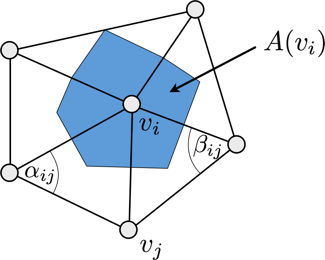
  • Solve \(\laplace_{\set{S}} \vec{u} = 0\) for all interior vertices \[\forall v_i \in \set{S} \setminus \partial\set{S} \;:\; \sum_{v_j \in \set{N}_1\of{v_i}} \big( \underbrace{\func{cot} \alpha_{ij} + \func{cot} \beta_{ij}}_{w_{ij}} \big) \left( \vec{u}\of{v_j} - \vec{u}\of{v_i} \right) = \vec{0} \]

Iterative Solution

  • Iterate until convergence
    • Solve condition for each interior vertex individually (keep \(w_{ij}\) fixed) \[ \forall v_i \in \set{S} \setminus \partial\set{S} \;:\; \vec{u}\of{v_i} \;\leftarrow\; \frac{1}{\sum_{v_j \in \set{N}_1\of{v_i}} w_{ij}} \sum_{v_j \in \set{N}_1\of{v_i}} w_{ij} \vec{u}\of{v_j}\]
  • Why does it converge? When does it converge?

Direct Solution

  • Assume that the vertices are partitioned/sorted into interior vertices \(v_1, \dots, v_n\) and boundary vertices \(v_{n+1}, \dots, v_{n+m}\)
  • Setup system of linear equations from the conditions for interior vertices and the boundary vertices \[ \matrix{ \rlap{\laplace_{n \times (n+m)}} \\ \mat{0}_{m \times n} & \mat{I}_{m \times m} } \cdot \matrix{ \vec{u}_1\T \\ \vdots \\ \vec{u}_n\T \\ \vec{u}_{n+1}\T \\ \vdots \\ \vec{u}_{n+m}\T } \;=\; \matrix{ \vec{0}\T \\ \vdots \\ \vec{0}\T \\ \bar{\vec{u}}_{n+1}\T \\ \vdots \\ \bar{\vec{u}}_{n+m}\T } \]

Direct Solution

  • Simplify this \((n+m) \times (n+m)\) system \[ \matrix{ \laplace_{n \times n} & \laplace_{n \times m} \\ \mat{0}_{m \times n} & \mat{I}_{m \times m} } \cdot \matrix{ \vec{u}_1\T \\ \vdots \\ \vec{u}_n\T \\ \vec{u}_{n+1}\T \\ \vdots \\ \vec{u}_{n+m}\T } \;=\; \matrix{ \vec{0}\T \\ \vdots \\ \vec{0}\T \\ \bar{\vec{u}}_{n+1}\T \\ \vdots \\ \bar{\vec{u}}_{n+m}\T } \]

  • Move the \(m\) known boundary vertices to right hand side
    (then we don’t need the bottom \(m\) rows anymore) \[ \laplace_{n \times n} \cdot \matrix{ \vec{u}_1\T \\ \vdots \\ \vec{u}_n\T } \;=\; \matrix{ \vec{0}\T \\ \vdots \\ \vec{0}\T } -\laplace_{n \times m} \matrix{ \bar{\vec{u}}_{n+1}\T \\ \vdots \\ \bar{\vec{u}}_{n+m}\T } \]

Direct Solution

  • This gives an \(n \times n\) linear system to solve for \(u\) and \(v\) coordinates. \[ \mat{D}\mat{M} \cdot \matrix{ \vec{u}_1\T \\ \vdots \\ \vec{u}_n\T } \;=\; \mat{D}\matrix{ \vec{b}_1\T \\ \vdots \\ \vec{b}_n\T } \]

\[ \mat{M}_{ij} \;=\; \begin{cases} \func{cot}\alpha_{ij} + \func{cot}\beta_{ij}, & i \ne j \,,\; j \in \set{N}_1\of{v_i} \setminus \partial\set{S} \\ -\sum_{v_j \in \set{N}_1\of{v_i}} \left( \func{cot}\alpha_{ij} + \func{cot}\beta_{ij} \right) & i=j \\ 0 & \text{otherwise} \end{cases} \]

\[\mat{D} = \func{diag}\of{ \dots, \frac{1}{2A_i}, \dots}\]

\[ \vec{b}_i \;=\; -\sum_{v_j \in \set{N}_1\of{v_i} \cap \partial\set{S} } \left( \func{cot}\alpha_{ij} + \func{cot}\beta_{ij} \right) \bar{\vec{u}}_j \]

Direct Solution

  • Let’s make it symmetric by removing \(\mat{D}\). Negating it makes it positive definite. \[ -\mat{M} \cdot \matrix{ \vec{u}_1\T \\ \vdots \\ \vec{u}_n\T } \;=\; -\matrix{ \vec{b}_1\T \\ \vdots \\ \vec{b}_n\T } \]

\[ \mat{M}_{ij} \;=\; \begin{cases} \func{cot}\alpha_{ij} + \func{cot}\beta_{ij}, & i \ne j \,,\; j \in \set{N}_1\of{v_i} \setminus \partial\set{S} \\ -\sum_{v_j \in \set{N}_1\of{v_i}} \left( \func{cot}\alpha_{ij} + \func{cot}\beta_{ij} \right) & i=j \\ 0 & \text{otherwise} \end{cases} \]

\[ \vec{b}_i \;=\; -\sum_{v_j \in \set{N}_1\of{v_i} \cap \partial\set{S} } \left( \func{cot}\alpha_{ij} + \func{cot}\beta_{ij} \right) \bar{\vec{u}}_j \]

Direct Solution

  • Solve sparse symmetric positive definite linear system \[ -\mat{M} \cdot \matrix{ \vec{u}_1\T \\ \vdots \\ \vec{u}_n\T } \;=\; -\matrix{ \vec{b}_1\T \\ \vdots \\ \vec{b}_n\T } \]

  • Allows for efficient linear system solvers

    • Iterative: Conjugate Gradients
    • Direct: Sparse Cholesky
    • more details later…

What about iterative solution?

  • Iterate until convergence
    • Solve condition for each interior vertex individually (keep \(w_{ij}\) fixed) \[ \forall v_i \in \set{S} \setminus \partial\set{S} \;:\; \vec{u}\of{v_i} \;\leftarrow\; \frac{1}{\sum_{v_j \in \set{N}_1\of{v_i}} w_{ij}} \sum_{v_j \in \set{N}_1\of{v_i}} w_{ij} \vec{u}\of{v_j}\]
  • Why does this work?
    • Update corresponds to one Gauss-Seidel iteration for \(\laplace\vec{u}=\vec{0}\).
    • When solving \(\mat{A}\vec{x}=\vec{b}\) iterate: \(x_i \leftarrow \frac{1}{a_{ii}} \left( b_i - \sum_{j \neq i} a_{ij} x_j \right)\)
    • Solves each condition/row individually, one after the other
    • Converges for diagonally dominant matrices: \(\abs{a_{ii}} \geq \sum_{j \neq i} \abs{a_{ij}}\)
    • Very simple, but very slow for larger matrices…

Wikipedia: Gauss-Seidel

Try it yourself!

Try it yourself!

Smoothing

Diffusion Flow

  • Diffusion equation \[\frac{\partial f}{\partial t} = \lambda \Delta f\]
    • \(\lambda\) is the diffusion constant
    • \(\Delta\) is the Laplace operator

Wikipedia: Diffusion Equation

Diffusion Flow

  • 2nd order elliptic PDE \[\frac{\partial f(x,y,t)}{\partial t} \;=\; \lambda \left( \frac{\partial^2 f(x,y,t)}{\partial x^2} + \frac{\partial^2 f(x,y,t)}{\partial y^2} \right)\]

  • Solve numerically

    • Discretize in space & time
    • Discretize time derivative
    • Discretize spatial derivatives

Diffusion Flow in 2D

Diffusion Flow on Meshes

  • Continuous PDE: \(\frac{\partial \vec{x}}{\partial t} \;=\; \lambda \Delta \vec{x}\)
  • Discretization: \(\vec{x}_i \leftarrow \vec{x}_i + \delta t \, \lambda \Delta \vec{x}_i\)
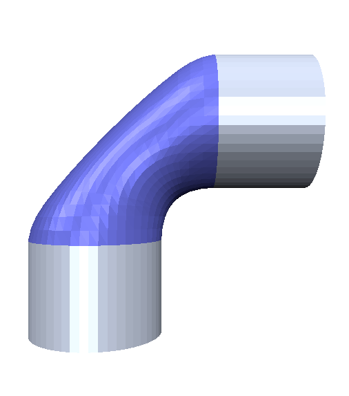
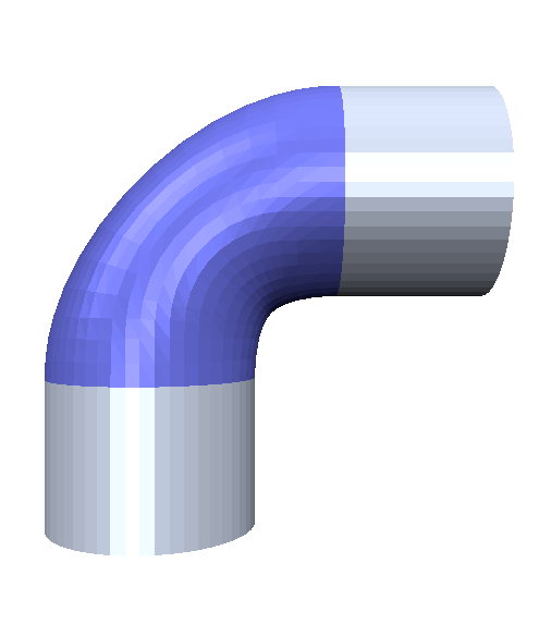
0 iterations
10 iterations
100 iterations

Explicit Integration

  • Use normalized weights and ignore the area term \[\vec{x}_i \leftarrow \vec{x}_i + \delta t \, \lambda \Delta \vec{x}_i\] \[\laplace \vec{x}_i \;=\; \frac{1}{\sum_{v_j \in \set{N}_1\of{v_i}} w_{ij}} \sum_{v_j \in \set{N}_1\of{v_i}} w_{ij} \left( \vec{x}_j - \vec{x}_i \right) \]
  • Largest stable time-step is \(\delta t \lambda = 1\), which yields \[\vec{x}_i \leftarrow \frac{1}{\sum_{v_j \in \set{N}_1\of{v_i}} w_{ij}} \sum_{v_j \in \set{N}_1\of{v_i}} w_{ij} \vec{x}_j\]
  • This is exactly one Gauss-Seidel iteration for \(\laplace\vec{x}=0\)!
    • Explicit integration will converge to this solution

Implicit Integration

  • Matrix version of implicit integration \[\left( \mat{I} - \delta t \laplace \right) \, \vec{X}^{(t+1)} = \vec{X}^{(t)}\]
  • Implicit integration works for any time-step!
  • Largest stable time-step is \(\infty\), which yields \[ \left( \frac{1}{\delta t}\vec{I} - \laplace \right) \, \vec{X}^{(t+1)} \;=\; \frac{1}{\delta t}\vec{X}^{(t)} \] \[ \underset{\delta t \to \infty}{\longrightarrow} \;\; -\laplace \, \vec{X}^{(t+1)} \;=\; \vec{0} \]
  • Implicit integration also converges to \(\laplace\vec{x}=\vec{0}\).
    • Very similar to parameterization!

Try it yourself!

Try it yourself!

Fairing

Fair Surfaces

  • Main idea:
    • Penalize “unaesthetic behavior”
    • Avoid unnecessary oscillations
    • Principle of the simplest shape
  • Minimize some fairness functional
    • Look for physical interpretation
    • Minimize surface area → membrane surface
    • Minimize curvature → thin plate surface

Membrane Surfaces

  • Minimize surface area \[\int_\set{S} \func{d}A \;\to\; \min \quad\text{with}\quad \delta\set{S}=\bar{\vec{x}}\]
  • Simpler energy using partial derivatives (Dirichlet energy) \[\int_\Omega \norm{\vec{x}_{,u}}^2 + \norm{\vec{x}_{,v}}^2 \func{d}u\func{d}v \;\to\;\min\]
  • Variational calculus gives \[ \begin{align} \laplace_{\set{S}} \vec{x} &= \vec{0}, & \vec{x} \in \set{S} \setminus \partial\set{S} \\ \vec{x} &= \bar{\vec{x}}, & \vec{x} \in \partial\set{S} \end{align} \]

Discretization

  • Assume that the vertices are partitioned/sorted into interior vertices \(v_1, \dots, v_n\) and boundary vertices \(v_{n+1}, \dots, v_{n+m}\) \[ \matrix{ \rlap{\laplace_{n \times (n+m)}} \\ \mat{0}_{m \times n} & \mat{I}_{m \times m} } \cdot \matrix{ \vec{x}_1\T \\ \vdots \\ \vec{x}_n\T \\ \vec{x}_{n+1}\T \\ \vdots \\ \vec{x}_{n+m}\T } \;=\; \matrix{ \vec{0}\T \\ \vdots \\ \vec{0}\T \\ \bar{\vec{x}}_{n+1}\T \\ \vdots \\ \bar{\vec{x}}_{n+m}\T } \]
  • Applying same tricks as for parameterization leads to \[ -\mat{M} \cdot \matrix{ \vec{x}_1\T \\ \vdots \\ \vec{x}_n\T } \;=\; -\matrix{ \vec{b}_1\T \\ \vdots \\ \vec{b}_n\T } \]

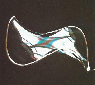
Membrane Surfaces aka Minimal Surface

  • Mean curvature \(H = \frac{\kappa_1 + \kappa_2}{2}\)
    • \(\laplace_{\set{S}} \vec{x} = -2 H \vec{n}\)
    • \(H = 0\) everywhere → membrane surface
    • \(\laplace_{\set{S}} \vec{x} = \vec{0}\) → smoothing stops
  • Connection to smoothing & parameterization
    • Membrane surfaces are stationary under smoothing
    • Smoothing converges to membrane surface
    • Parameterization also minimizes area, but flattens boundary first
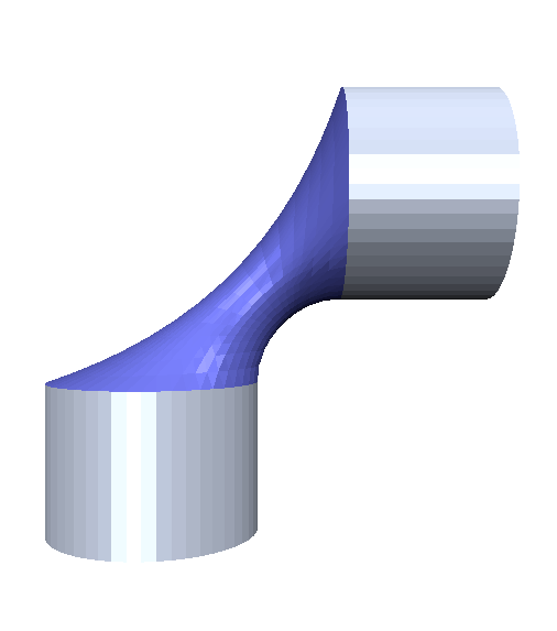
Wikipedia: Minimal Surface

Try it yourself!

Try it yourself!

Thin Plate Surfaces

  • Minimize surface curvature \[\int_\set{S} \kappa_1^2 + \kappa_2^2 \,\func{d}A \to \min \;\text{with}\; \begin{cases} \delta\set{S}=\bar{\vec{x}} \\ \vec{n}\of{\delta\set{S}}=\bar{\vec{n}} \end{cases}\]
  • Simpler energy using partial derivatives
    (thin plate energy) \[\int_\Omega \norm{\vec{x}_{,uu}}^2 + 2\norm{\vec{x}_{,uv}}^2 + \norm{\vec{x}_{,vv}}^2 \func{d}u\func{d}v \;\to\;\min\]
  • Variational calculus gives \[\begin{align} \laplace_{\set{S}}^2 \vec{x} &= \vec{0}, & \vec{x} \in \set{S} \setminus \partial\set{S} \\ \vec{x} &= \bar{\vec{x}}, & \vec{x} \in \partial\set{S} \\ \vec{n}\of{\vec{x}} &= \bar{\vec{n}}, & \vec{x} \in \partial\set{S} \\ \end{align}\]
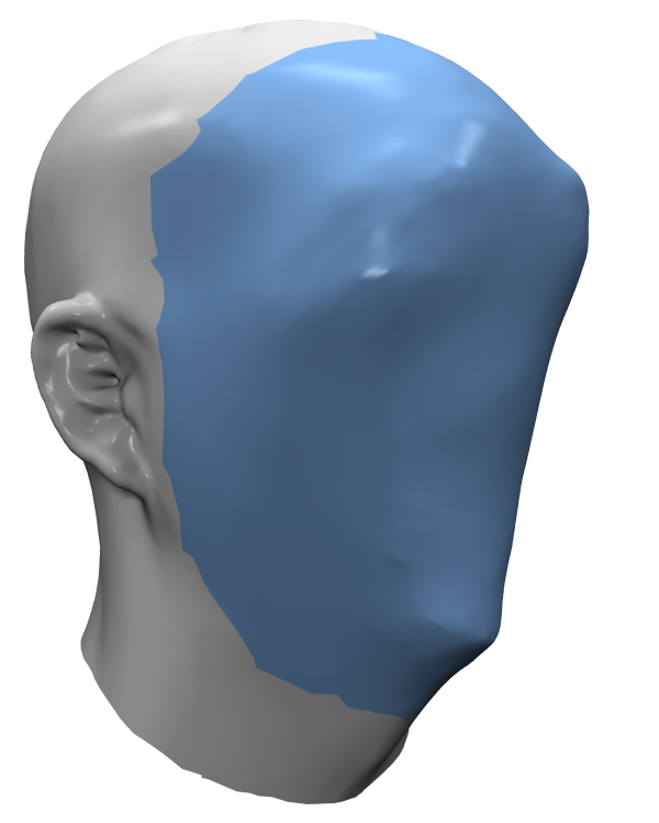
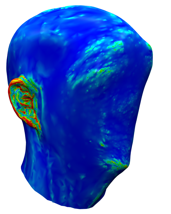
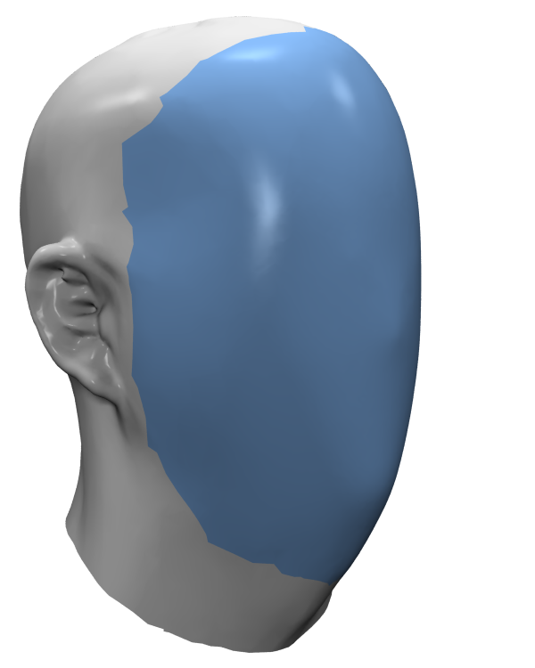
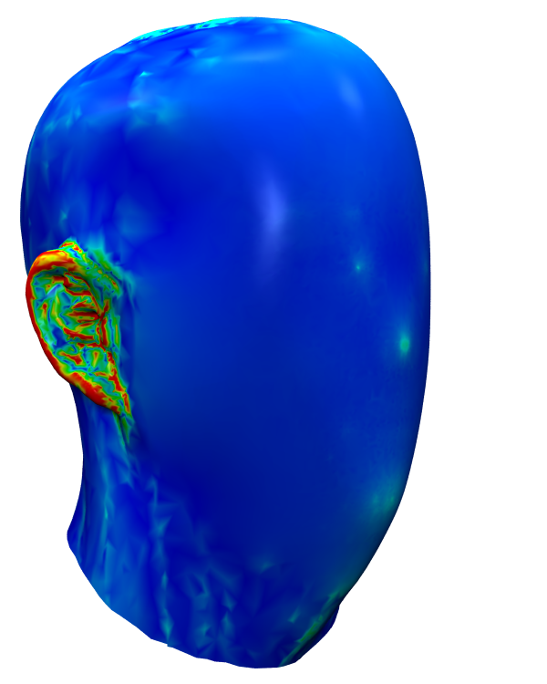
Discretization

  • Assume that the vertices are partitioned into interior vertices \(v_1, \dots, v_n\) and two rings of boundary vertices \(v_{n+1}, \dots, v_{n+m}\) \[ \matrix{ \rlap{\laplace_{n \times (n+m)}^2} \\ \mat{0}_{m \times n} & \mat{I}_{m \times m} } \cdot \matrix{ \vec{x}_1\T \\ \vdots \\ \vec{x}_n\T \\ \vec{x}_{n+1}\T \\ \vdots \\ \vec{x}_{n+m}\T } \;=\; \matrix{ \vec{0}\T \\ \vdots \\ \vec{0}\T \\ \bar{\vec{x}}_{n+1}\T \\ \vdots \\ \bar{\vec{x}}_{n+m}\T } \]
  • Recursive Laplace discretization \[ \laplace^2 f\of{v_i} \;=\; \laplace\of{\laplace f\of{v_i}} \;=\; \frac{1}{2 A_i} \sum_{v_j \in \set{N}_1\of{v_i}} \left( \func{cot} \alpha_{ij} + \func{cot} \beta_{ij} \right) \left( \laplace f \of{v_j} - \laplace f \of{v_i} \right) \]

Discretization

  • Assume that the vertices are partitioned into interior vertices \(v_1, \dots, v_n\) and two rings of boundary vertices \(v_{n+1}, \dots, v_{n+m}\) \[ \matrix{ \rlap{\laplace_{n \times (n+m)}^2} \\ \mat{0}_{m \times n} & \mat{I}_{m \times m} } \cdot \matrix{ \vec{x}_1\T \\ \vdots \\ \vec{x}_n\T \\ \vec{x}_{n+1}\T \\ \vdots \\ \vec{x}_{n+m}\T } \;=\; \matrix{ \vec{0}\T \\ \vdots \\ \vec{0}\T \\ \bar{\vec{x}}_{n+1}\T \\ \vdots \\ \bar{\vec{x}}_{n+m}\T } \]
  • Move fixed vertices to right hand side and remove one \(\mat{D}\) \[ \mat{M}\mat{D}\mat{M} \cdot \matrix{ \vec{x}_1\T \\ \vdots \\ \vec{x}_n\T } \;=\; \matrix{ \vec{b}_1\T \\ \vdots \\ \vec{b}_n\T } \]

Energy Functionals

Membrane surface
\[\laplace_{\set{S}} \vec{x} = 0\]

Thin plate surface
\[\laplace_{\set{S}}^2 \vec{x} = 0\]

Minimum variation surface
\[\laplace_{\set{S}}^3 \vec{x} = 0\]

Try it yourself!

Try it yourself!

Try it yourself!

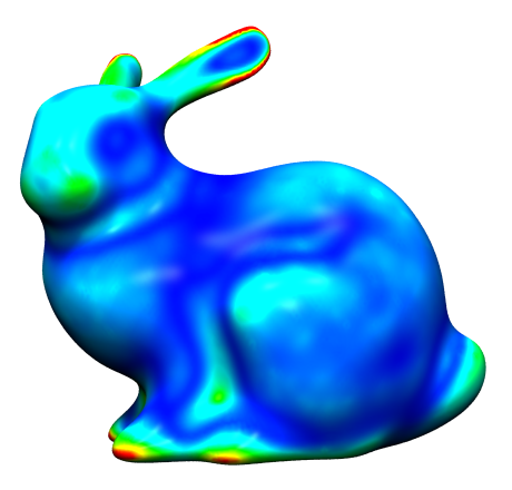
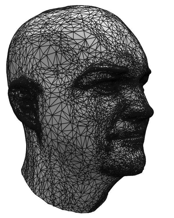
Laplace discretization matters!

original

uniform Laplace

cotan Laplace

Linear System Solvers

  • Solvers for sparse symmetric positive definite systems?
  • Dense Cholesky factorization
    • Cubic complexity, high memory consumption
  • Iterative conjugate gradients
    • Quadratic complexity, low memory consumption
  • Multigrid solvers
    • Linear complexity, but complicated to use
  • Sparse Cholesky factorization
    • Almost linear complexity and very easy to use!

Benchmark: Laplace Systems

Benchmark: Laplace Systems

Benchmark: Laplace2 Systems

Benchmark: Laplace2 Systems

Literature

  • Botsch et al., Polygon Mesh Processing, AK Peters, 2010
    • Chapter 4: Smoothing & Fairing
    • Appendix A: Numerics

  • Desbrun, Meyer, Schröder, Barr: Implicit Fairing of Irregular Meshes using Diffusion and Curvature Flow, SIGGRAPH 1999

  • Desbrun, Meyer, Alliez: Intrinsic Parameterizations of Surface Meshes, Eurographics 2002

  • Jacobson, Tosun, Sorkine, Zorin: Mixed Finite Elements for Variational Surface Modeling, SGP 2010.