Lecture 3D Geometry Processing
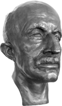
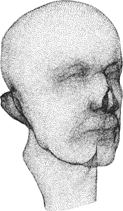
Surface Reconstruction
Prof. Dr. David Bommes
Computer Graphics Group
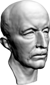
Surface Reconstruction
Advantages
result is closed 2-manifold surface
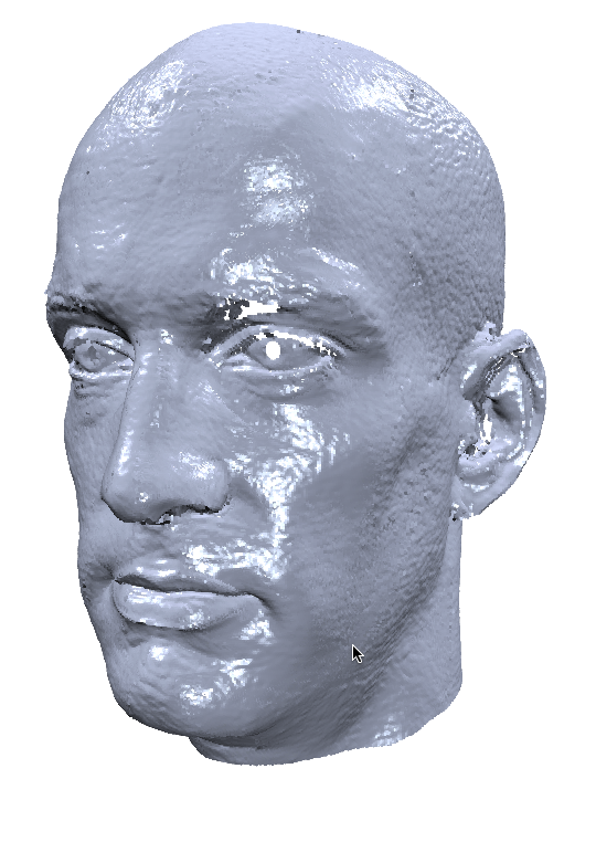
suitable for noisy input data
Recall: 2D Marching Squares Algorithm
Classify grid nodes as inside/outside
Is \(F(x_{i,j})\) below or above iso-value?
Classify cell: \(2^4 = 16\) configurations
Determine contour edges
look-up table for edge configuration
Determine vertex positions
linear interpolation of grid values along edges
Recall: 2D Marching Squares Algorithm
3D Marching Cubes Algorithm
Classify grid nodes as inside/outside
Is \(F(x_{i,j,k})\) below or above iso-value?
Classify cell: \(2^8 = 256\) configurations
Determine contour triangles
look-up table for triangle configuration
Determine vertex positions
linear interpolation of grid values along edges
3D Marching Cubes Algorithm
Poisson Surface Reconstruction
Slides courtesy of Misha Kazhdan
Source Code available at:
http://www.cs.jhu.edu/~misha/
Implementation included in Meshlab and many other tools
Misha Kazhdan
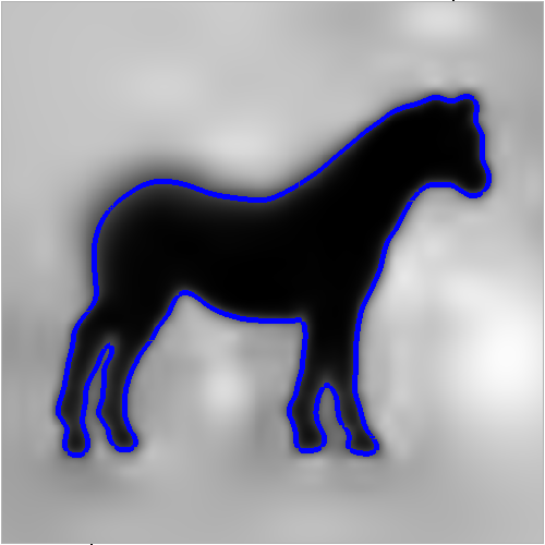
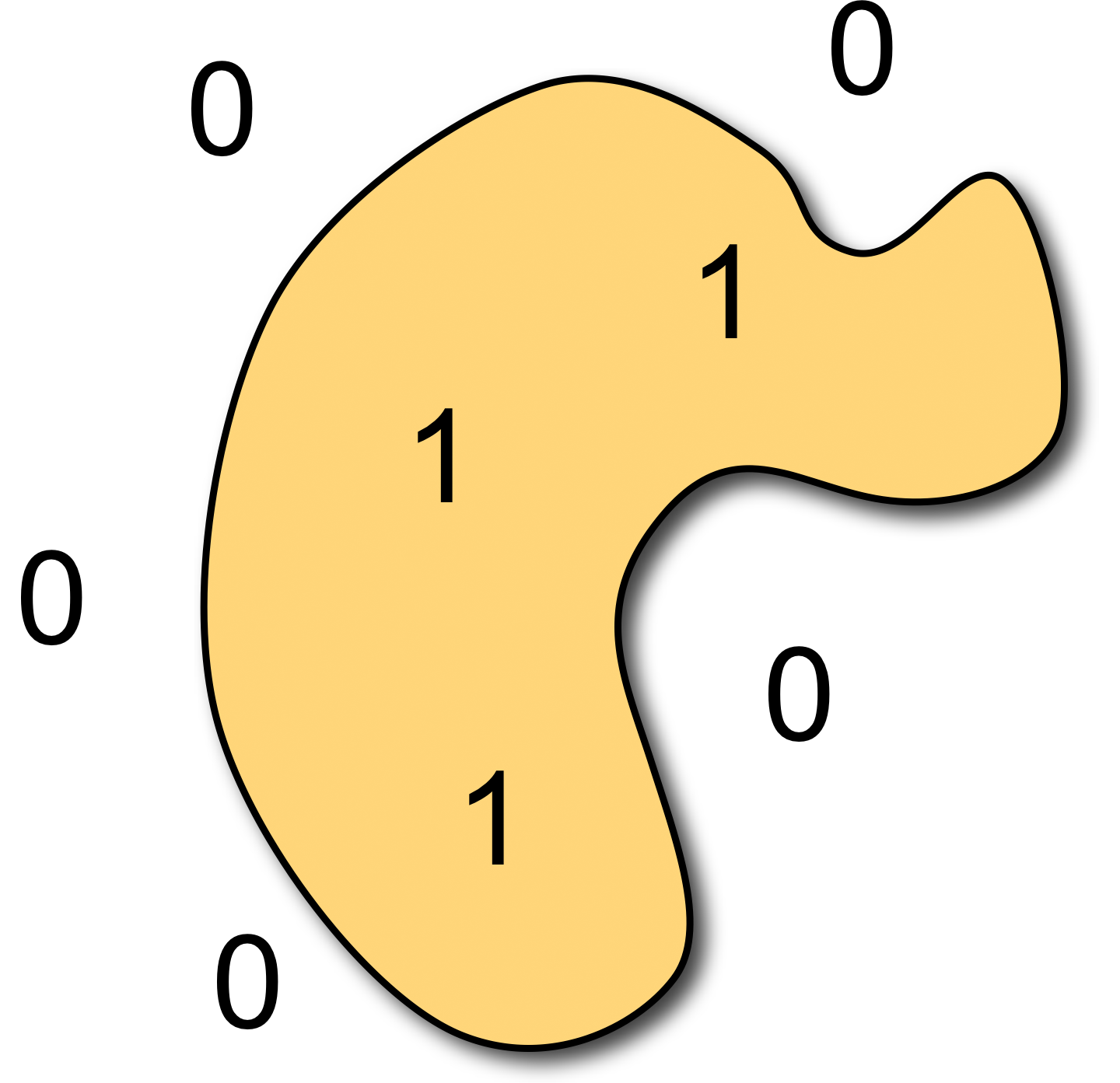
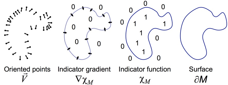
The Indicator Function
We reconstruct the surface of the model by solving for the indicator function \(\chi\) of the shape
\[\chi(\vec{p}) \;=\;
\begin{cases}
1 & \text{if } \vec{p} \in \set{M} \\
0 & \text{if } \vec{p} \not\in \set{M} \\
\end{cases}\]
Indicator function \(\chi\)
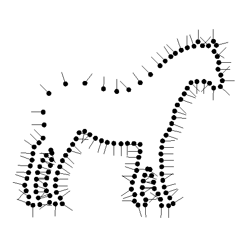
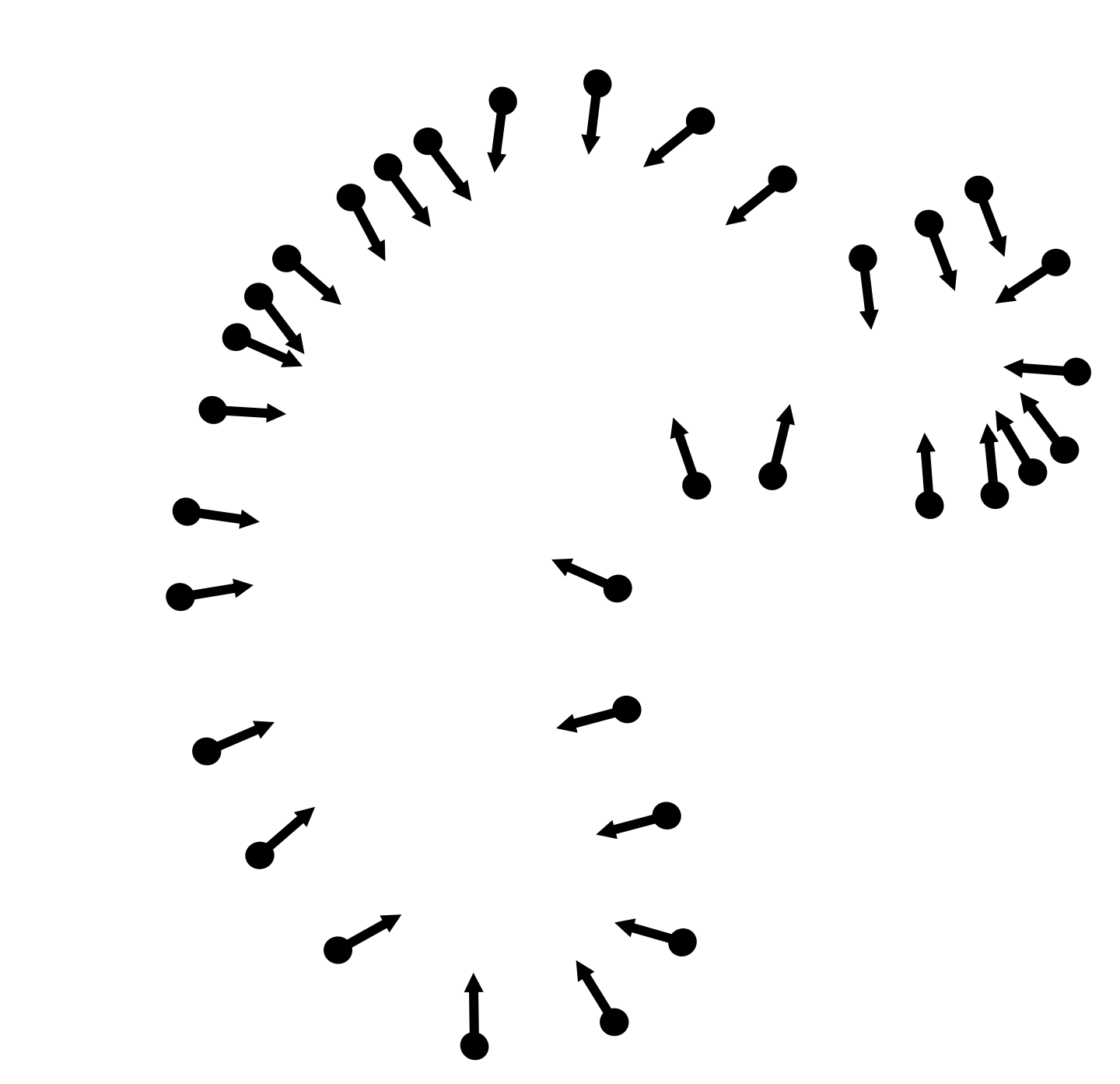
Challenge
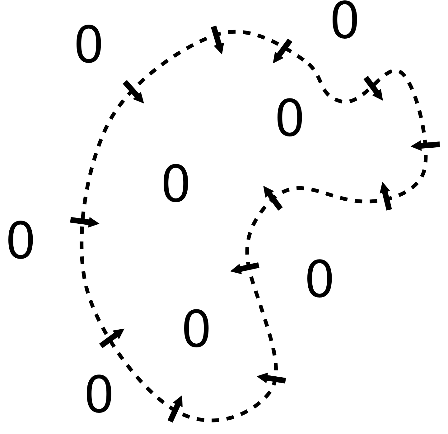
How to construct the indicator function from a set of oriented points?
Oriented points Indicator function \(\chi\)
Gradient Relationship
There is a relationship between the normal field and gradient of (smoothed) indicator function
Oriented points Indicator gradient \(\nabla \chi\)
Recap: Notation
\[u\of{\vec{x}} \;=\; u(x,y,z)\]
\[\vec{u}\of{\vec{x}} \;=\;
\vector{ u(\vec{x}) \\ v(\vec{x}) \\ w(\vec{x}) } \;=\;
\vector{ u(x,y,z) \\ v(x,y,z) \\ w(x,y,z) }\]
Recap: Notation
\[\grad u\of{\vec{x}} =
\vector{
\diff{u}{x}\of{\vec{x}} \\[1mm]
\diff{u}{y}\of{\vec{x}} \\[1mm]
\diff{u}{z}\of{\vec{x}}
}
\,,\quad
\grad \vec{u}\of{\vec{x}} =
\matrix{
\diff{u}{x}\of{\vec{x}} & \diff{u}{y}\of{\vec{x}} & \diff{u}{z}\of{\vec{x}} \\[1mm]
\diff{v}{x}\of{\vec{x}} & \diff{v}{y}\of{\vec{x}} & \diff{v}{z}\of{\vec{x}} \\[1mm]
\diff{w}{x}\of{\vec{x}} & \diff{w}{y}\of{\vec{x}} & \diff{w}{z}\of{\vec{x}}
}\]
Recap: Notation
Gradient & Jacobian, simplified notation
\[\grad u\of{\vec{x}} =
\vector{
u_{,x}\of{\vec{x}} \\
u_{,y}\of{\vec{x}} \\
u_{,z}\of{\vec{x}}
}
\,,\quad
\grad \vec{u}\of{\vec{x}} =
\matrix{
u_{,x}\of{\vec{x}} & u_{,y}\of{\vec{x}} & u_{,z}\of{\vec{x}} \\
v_{,x}\of{\vec{x}} & v_{,y}\of{\vec{x}} & v_{,z}\of{\vec{x}} \\
w_{,x}\of{\vec{x}} & w_{,y}\of{\vec{x}} & w_{,z}\of{\vec{x}}
}
\]
comma-subindex denotes the partial derivative
Recap: Notation
\[\func{div}\of{\vec{u}}\of{\vec{x}} =
\left( \grad \cdot \vec{u} \right) \of{\vec{x}} =
u_{,x}\of{\vec{x}} + v_{,y}\of{\vec{x}} + w_{,z}\of{\vec{x}}\]
\[\left( \grad \cdot \vec{u} \right) =
\vector{
\diff{}{x} \\[1mm]
\diff{}{y} \\[1mm]
\diff{}{z}
}
\cdot
\vector{
u\of{\vec{x}} \\[1mm]
v\of{\vec{x}} \\[1mm]
w\of{\vec{x}}
}
\]
Recap: Notation
Gradient, Jacobian
\[\grad u\of{\vec{x}} =
\vector{
u_{,x}\of{\vec{x}} \\
u_{,y}\of{\vec{x}} \\
u_{,z}\of{\vec{x}}
}
\,,\quad
\grad \vec{u}\of{\vec{x}} =
\matrix{
u_{,x}\of{\vec{x}} & u_{,y}\of{\vec{x}} & u_{,z}\of{\vec{x}} \\
v_{,x}\of{\vec{x}} & v_{,y}\of{\vec{x}} & v_{,z}\of{\vec{x}} \\
w_{,x}\of{\vec{x}} & w_{,y}\of{\vec{x}} & w_{,z}\of{\vec{x}}
}
\]
Divergence
\[\func{div}\of{\vec{u}}\of{\vec{x}} =
\left( \grad \cdot \vec{u} \right) \of{\vec{x}} =
u_{,x}\of{\vec{x}} + v_{,y}\of{\vec{x}} + w_{,z}\of{\vec{x}}\]
Laplace
\[\laplace\vec{u}\of{\vec{x}} \;=\;
\grad^2\vec{u}\of{\vec{x}} \;=\;
\grad \cdot \grad\vec{u}\of{\vec{x}} \;=\;
\vec{u}_{,xx}\of{\vec{x}} + \vec{u}_{,yy}\of{\vec{x}} + \vec{u}_{,zz}\of{\vec{x}}\]
Recap: Notation
Gradient, Jacobian
\[
\grad u =
\vector{
u_{,x} \\
u_{,y} \\
u_{,z}
}
\,,\quad
\grad \vec{u} =
\matrix{
u_{,x} & u_{,y} & u_{,z} \\
v_{,x} & v_{,y} & v_{,z} \\
w_{,x} & w_{,y} & w_{,z}
}
\]
Divergence
\[\func{div}\of{\vec{u}} =
\grad \cdot \vec{u} =
u_{,x} + v_{,y} + w_{,z}
\]
Laplace
\[\laplace\vec{u} \;=\;
\grad^2\vec{u} \;=\;
\grad \cdot \grad\vec{u} \;=\;
\vec{u}_{,xx} + \vec{u}_{,yy} + \vec{u}_{,zz}
\]
Integration as a Poisson Problem
Approximate gradients by a vector field \(\vec{v}(\vec{x})\)
\(\vec{v}(\vec{x}) = \vec{0}\;\) inside and outside\(\vec{v}(\vec{p}_i) = \vec{n}_i\;\) at point samples \(\vec{p}_i\) vector field equals point normals \(\vec{n}_i\)
Find indicator function \(\chi\) whose gradient best approximates \(\vec{v}\) \[\min_{\chi} \int \norm{ \grad\chi (\vec{x}) - \vec{v} (\vec{x})}^2 \func{d}x\]
not every vector field is integrable, i.e. can be represented as the gradient of a scalar function
Variational calculus leads to Poisson equation \[\laplace \chi \;=\; \grad \cdot \vec{v}\]
Variational Calculus in 1D
Minimize deviation from \(v(x)\) on interval \([a,b]\) \[C(f) = \int_a^b \left( f'(x) - v(x) \right)^2 \func{d}x \;\to\;\min\]
Add test function \(u\) with \(u(a) = u(b) = 0\) \[C\of{f+\lambda u} =
\int_a^b \left( f' + \lambda u' - v\right)^2 \func{d}x =
\int_a^b \lambda^2 {u'}^2 + 2\lambda (f'-v) u' + \left({f'}-v\right)^2 \func{d}x
\]
If f minimizes C, the following has to vanish \[
\left.
\frac{\partial C\of{f+\lambda u}}{\partial \lambda}
\right|_{\lambda=0}
\;=\;
\int_a^b 2 (f'-v) u' \, \func{d}x
\;\stackrel{!}{=}\;
0
\]
Variational Calculus in 1D
Has to vanish for any \(u\) with \(u(a) = u(b) = 0\) \[
\int_a^b (f'-v)u' \, \func{d}x
\;=\;
\underbrace{\left[ (f'-v) u \right]_a^b}_{=0} -
\int_a^b (f''-v')u \, \func{d}x
\;\stackrel{!}{=}\;
0
\quad \forall u
\]
Only possible if \[
f'' - v' \;=\; 0 \quad\Leftrightarrow\quad \laplace f = \grad \cdot v
\]
So-called Euler-Lagrange Equation
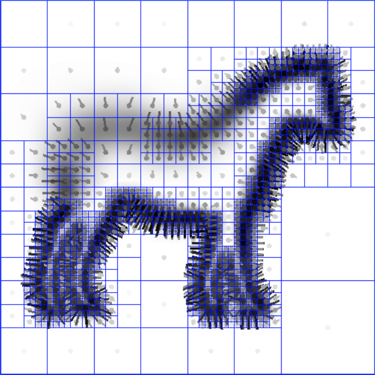
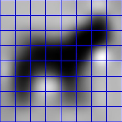
Implementation
Given the input point set:
Setup adaptive octree
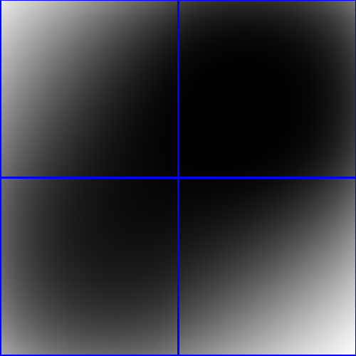
Compute vector field
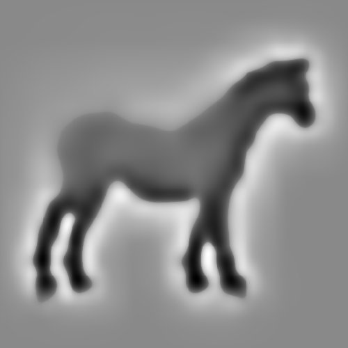
Compute indicator function
Extract iso-surface
Implementation
Given the input point set:
Setup adaptive octree Compute vector field
Compute indicator function
Extract iso-surface
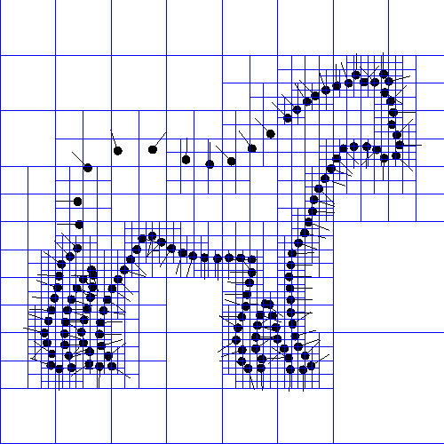
Implementation
Given the input point set:
Setup adaptive octree
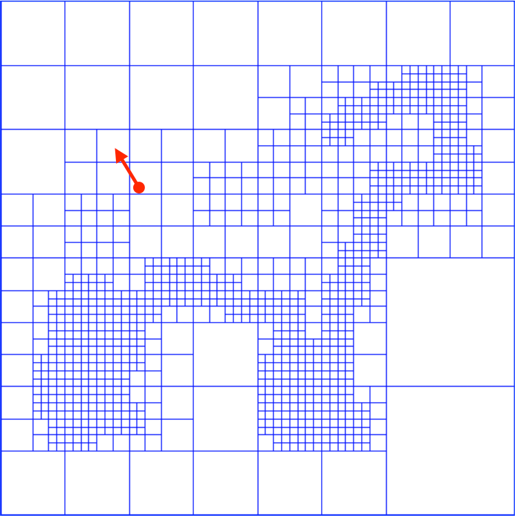
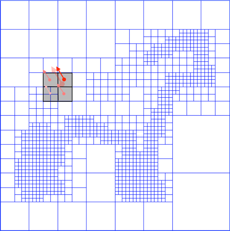
Compute vector field
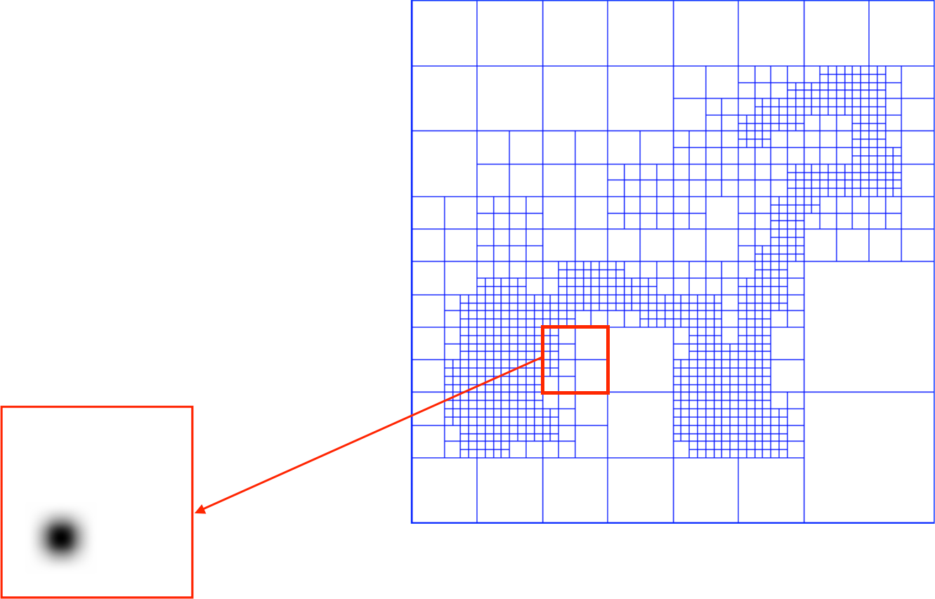
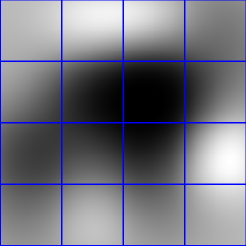
Define function basis Splat the samples
Compute indicator function
Extract iso-surface
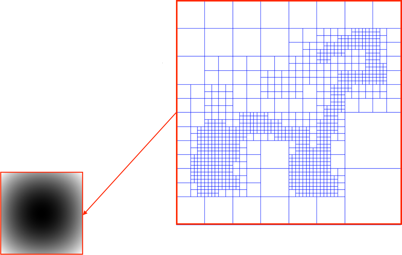
Implementation
Given the input point set:
Setup adaptive octree
Compute vector field
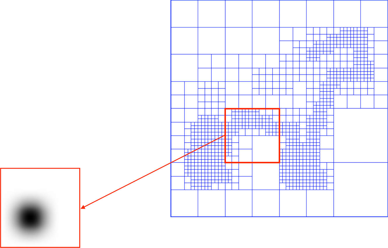
Define function basis
Splat the samples
Compute indicator function
Extract iso-surface
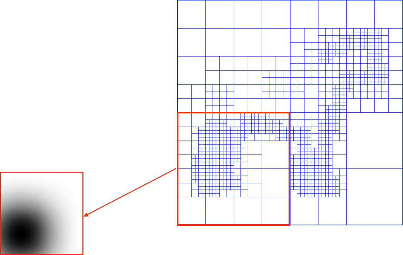
Implementation
Given the input point set:
Setup adaptive octree
Compute vector field
Define function basis
Splat the samples
Compute indicator function
Extract iso-surface
Implementation
Given the input point set:
Setup adaptive octree
Compute vector field
Define function basis
Splat the samples
Compute indicator function
Extract iso-surface
Implementation
Given the input point set:
Setup adaptive octree
Compute vector field
Compute indicator function
Compute divergence Solve Poisson equation
Extract iso-surface
Implementation
Given the input point set:
Setup adaptive octree
Compute vector field
Compute indicator function
Extract iso-surface
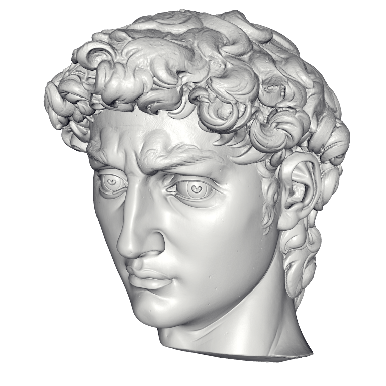
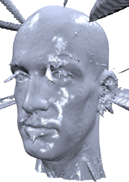
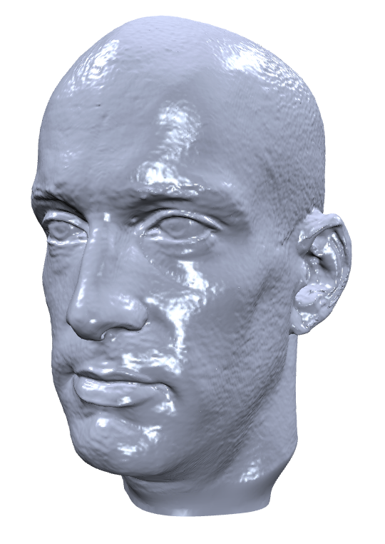
Poisson Surface Reconstruction
Summary
Poisson Surface Reconstruction
robustness to outliers
fills holes
performance through octree and multilevel solver
can also be implemented on tetrahedral mesh (CGAL implementation )