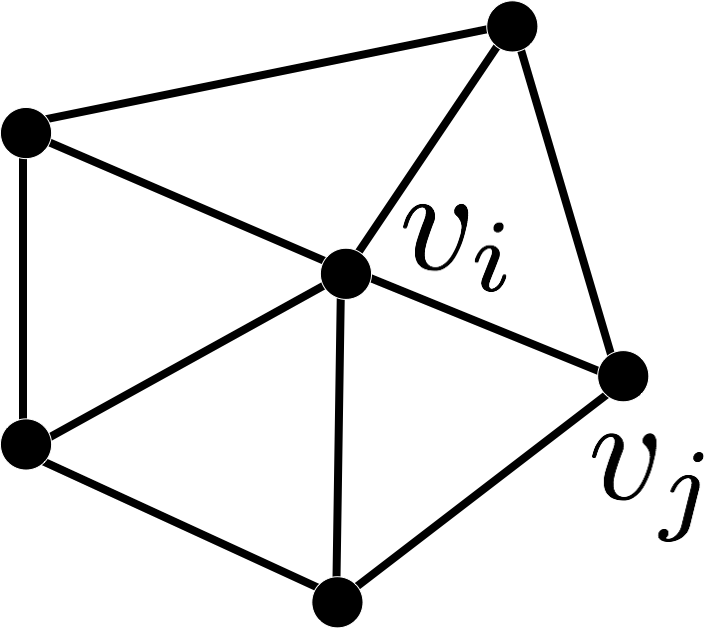
Triangle Meshes
- Connectivity / Topology
- Vertices \(\mathcal{V} = \{ v_1, \dots, v_n \}\)
- Edges \(\mathcal{E} = \{ e_1, \dots, e_k \}\), \(e_i \in \mathcal{V} \times \mathcal{V}\)
- Faces \(\mathcal{F} = \{ f_1, \dots, f_m \}\), \(f_i \in \mathcal{V} \times \mathcal{V} \times \mathcal{V}\)
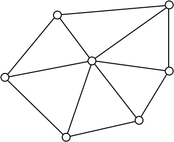
- Geometry
- Vertex positions \(\{ \vec{p}_1, \dots, \vec{p}_n \}\), \(\vec{p}_i \in \R^3\)
Why Triangle Meshes?
- Triangle meshes can represent arbitrary surfaces
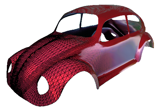
Why Triangle Meshes?
- Triangle meshes can represent arbitrary surfaces
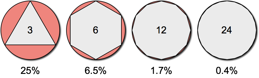
- Piecewise linear approximation → error is \(\mathcal{O}(h^2)\)
Why Triangle Meshes?
- Triangle meshes can represent arbitrary surfaces
- Piecewise linear approximation → error is \(\mathcal{O}(h^2)\)
- Approximation error inversely proportional to #triangles
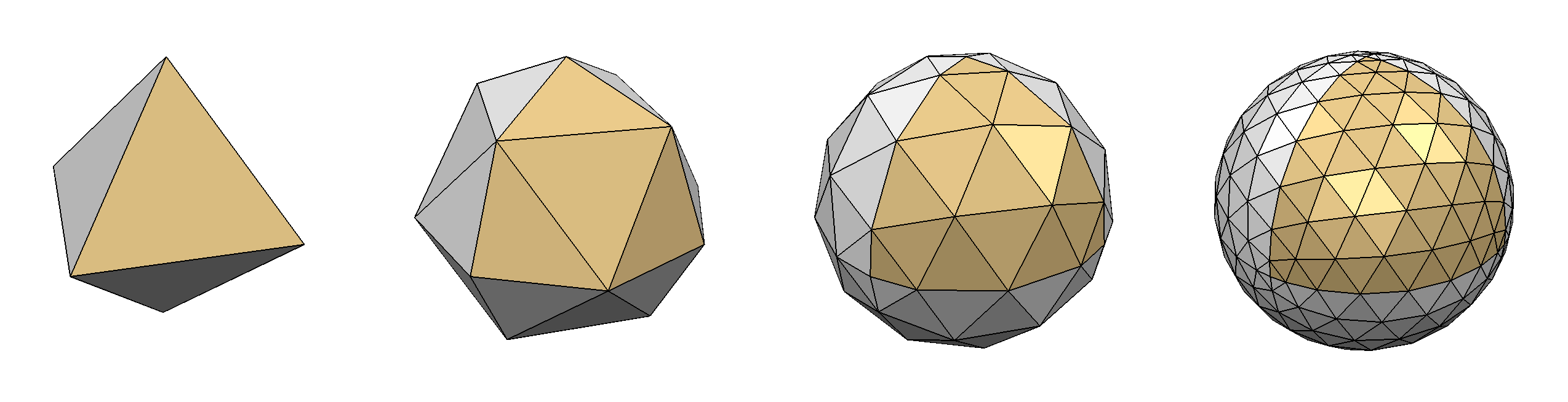
Why Triangle Meshes?
- Triangle meshes can represent arbitrary surfaces
- Piecewise linear approximation → error is \(\mathcal{O}(h^2)\)
- Approximation error inversely proportional to #triangles
- Adaptive tesselation can adapt to surface curvature
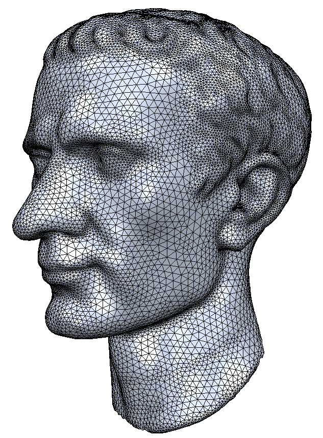
Why Triangle Meshes?
- Triangle meshes can represent arbitrary surfaces
- Piecewise linear approximation → error is \(\mathcal{O}(h^2)\)
- Approximation error inversely proportional to #triangles
- Adaptive tesselation can adapt to surface curvature
- Simple primitives can be processed efficiently by CPU/GPU
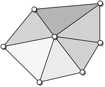
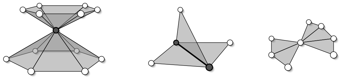
Two-Manifold Surfaces
- Local neighborhoods are disk-shaped
- Guarantees meaningful neighborhood enumeration
- Required by most algorithms
- Non-manifold examples:
Face Set
- Face Set is a standard file format for triangle meshes (e.g. STL format)
- Memory consumption
36 B/f = 72 B/v

Indexed Face Set
- Indexed Face Sets are used for many file formats (e.g. OFF, OBJ, VRML)
- Memory consumption
12 B/v + 12 B/f = 36 B/v

Face-Based Connectivity
- Store connectivity per face
- Memory consumption
16 B/v + 24 B/f = 64 B/v - Non-constant element size for general polygonal meshes
- Edges not represented

Edge-Based Connectivity
- Store connectivity per edge
- Memory consumption
16 B/v + 4 B/f + 32 B/e = 120 B/v - Edges explicitly represented
- Missing edge orientation leads to case distinctions during traversal

Halfedge-Based Connectivity
- Store connectivity per halfedge
- Memory consumption
16 B/v + 4 B/f + 20 B/h = 144 B/v
(can be reduced to 96 B/v) - Edges & halfedges explicitly represented
- No case distinctions during traversal!

One-Ring Traversal
- Simple one-ring traversal without case distinctions:
- Start at vertex
- Outgoing halfedge
- Opposite halfedge
- Next halfedge
- Opposite halfedge
- Next halfedge
- …

Triangle Meshes
- Connectivity / Topology
- Vertices \(\mathcal{V} = \{ v_1, \dots, v_n \}\)
- Edges \(\mathcal{E} = \{ e_1, \dots, e_k \}\), \(e_i \in \mathcal{V} \times \mathcal{V}\)
- Faces \(\mathcal{F} = \{ f_1, \dots, f_m \}\), \(f_i \in \mathcal{V} \times \mathcal{V} \times \mathcal{V}\)
- Geometry
- Vertex positions \(\{ \vec{p}_1, \dots, \vec{p}_n \}\), \(\vec{p}_i \in \R^3\)
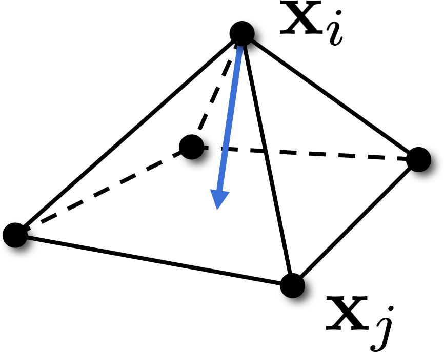
Normal Vectors
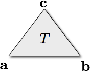
- Triangle normal \[ \vec{n}(T) = \frac{\left(\vec{b}-\vec{a}\right) \times \left(\vec{c}-\vec{a}\right)} {\norm{\left(\vec{b}-\vec{a}\right) \times \left(\vec{c}-\vec{a}\right)}} \]
- Vertex normal
- Average of incident triangles’ normals \(\vec{n}(T_i)\)
- Weighted by area or opening angle \(w(T_i)\)
Vertex Normals

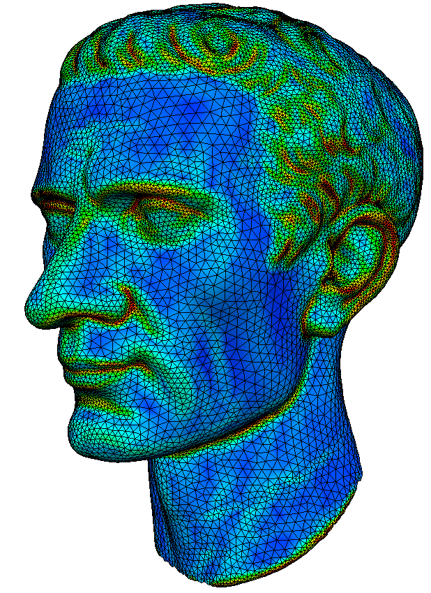
Discrete Curvatures
- How to discretize curvatures on a mesh?
- Zero curvature within triangles
- Infinite curvature at edges / vertices
- Point-wise definition does not make sense
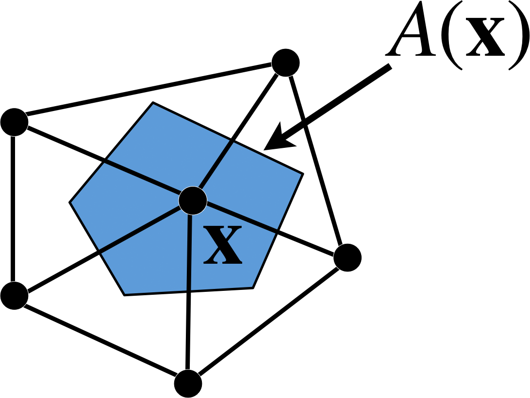
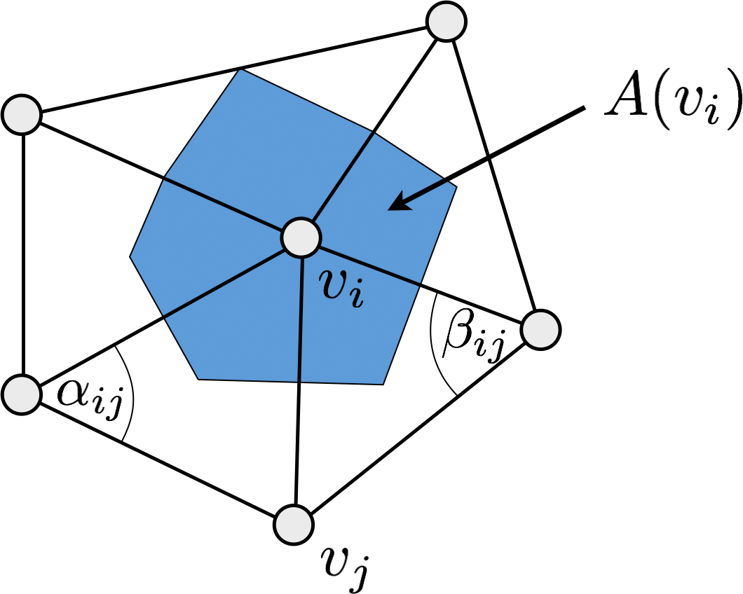
- Approximate differential properties at point \(\vec{x}\) as average over local neighborhood \(A(\vec{x})\)
- \(\vec{x}\) is a mesh vertex
- \(A(\vec{x})\) is within one-ring neighborhood
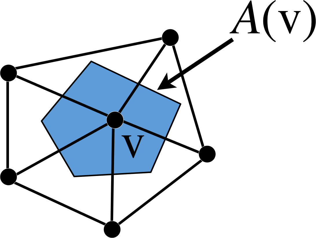
Discrete Curvatures
- How to discretize curvatures on a mesh?
- Zero curvature within triangles
- Infinite curvature at edges / vertices
- Point-wise definition does not make sense
- Approximate differential properties at vertex \(v\) as average over local neighborhood \(A(v)\) \[C\of{v} \;\approx\; \frac{1}{A\of{v}} \int_{A\of{v}} C\of{\vec{x}} \func{d}A\]
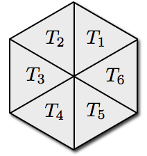
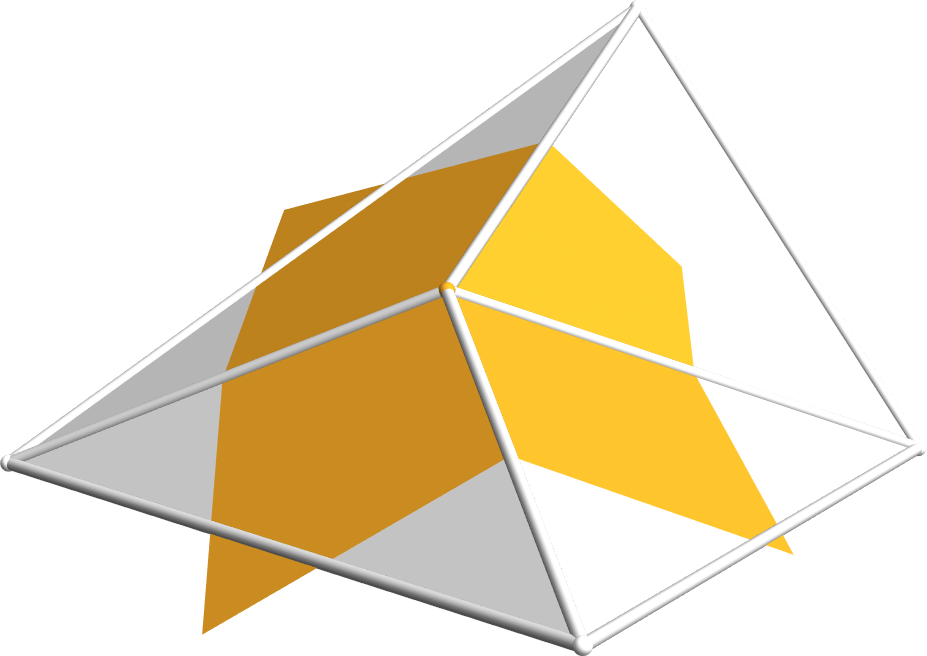
Barycentric Cells
- For each triangle of one-ring, connect vertex with edge midpoints and triangle barycenters
- Simple to compute: Area is 1/3 of triangle areas
- How to compute triangle areas?
3D Cross Product
- Given two 3D vectors \(\vec{a}\) and \(\vec{b}\), computes a vector \(\vec{c}\) that is orthogonal to them \[ \vec{c} \;=\; \vec{a} \times \vec{b} \;=\; {\tiny \matrix{ a_2 b_3 - a_3 b_2 \\ a_3 b_1 - a_1 b_3 \\ a_1 b_2 - a_2 b_1 }} \]
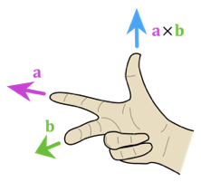
- Measures the area of parallelogram spanned by vectors \(\vec{a}\) and \(\vec{b}\) \[ \norm{\vec{a} \times \vec{b}} = \norm{\vec{a}} \cdot \norm{\vec{b}} \cdot \sin\theta \]
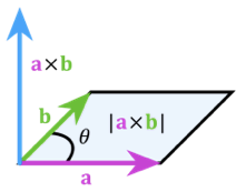
- Measures volume spanned by vectors \(\vec{a}\), \(\vec{b}\), \(\vec{c}\) \[ \mathrm{vol}\of{\vec{a}, \vec{b}, \vec{c}} \;=\; \abs{ \vec{a} \, \vec{b} \, \vec{c} } \;=\; \trans{\left( \vec{a} \times \vec{b} \right)} \vec{c} \]
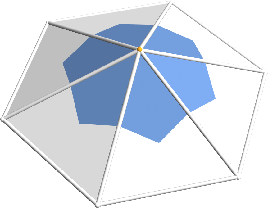
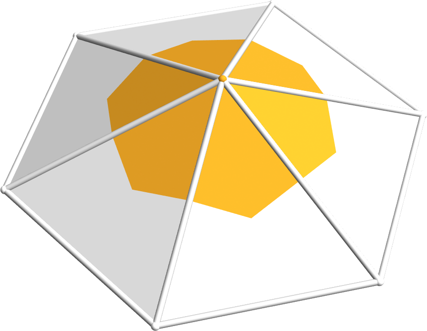
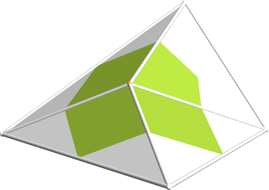
Voronoi Cells
- For each triangle of one-ring, connect vertex with edge midpoints and triangle circumcenter
- How to compute circumcircles?
- see discrete osculating circle exercise
Barycentric vs. Voronoi Cells
Voronoi cells provide better approximation than barycentric cells, but are more complex to compute
barycentric voronoi 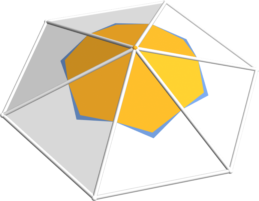
comparison 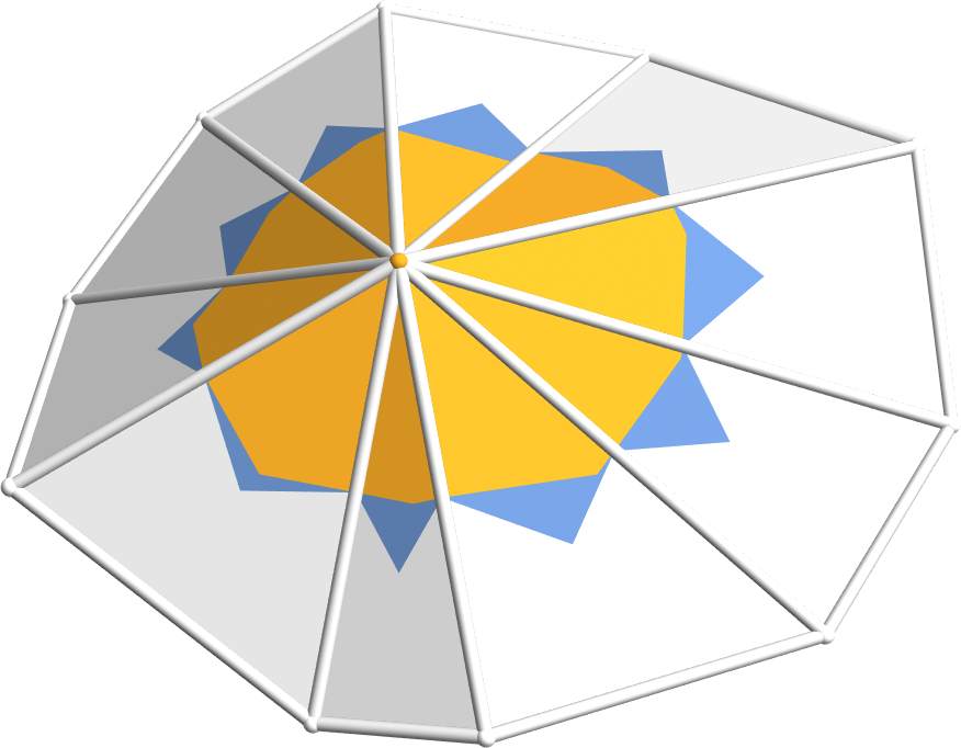
comparison
- Problem: Circumcenter can lie outside of triangle
Mixed Cells
- For each triangle of one-ring, connect vertex with edge midpoints and …
- … circumcenters for non-obtuse triangles
- … midpoints of opposite edge for obtuse triangles

- See Meyer et al. 2003 for computational details.
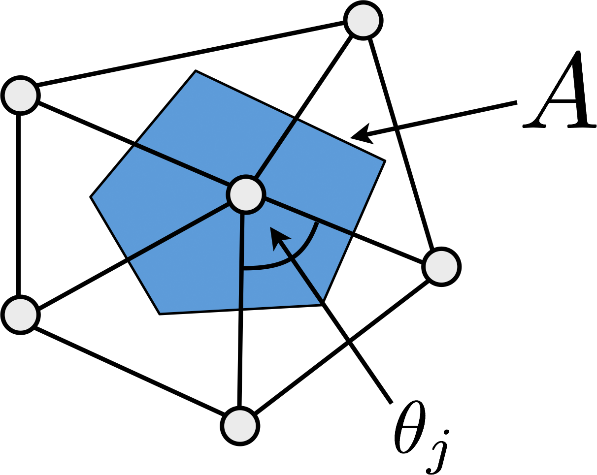
Discrete Gauss Curvature
- Compute Gauss curvature by Gauss-Bonnet theorem and averaging
\[ K(v) \approx \frac{1}{| A(v) |} \int_{A(v)} K \, dA = \frac{1}{| A(v) |} \left( 2 \pi - \sum_j \theta_{j} \right)\]
Laplace Operator on Meshes?
- Extend finite differences to meshes? Which weights to choose per vertex / edge?
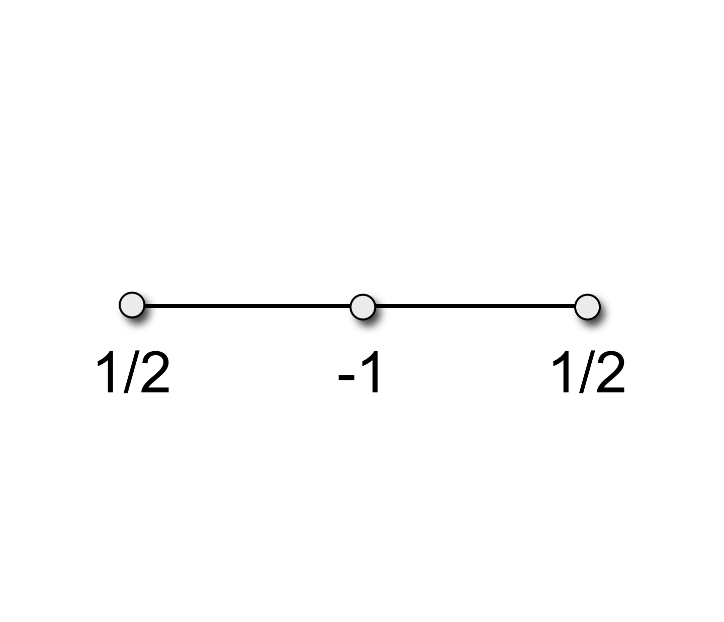
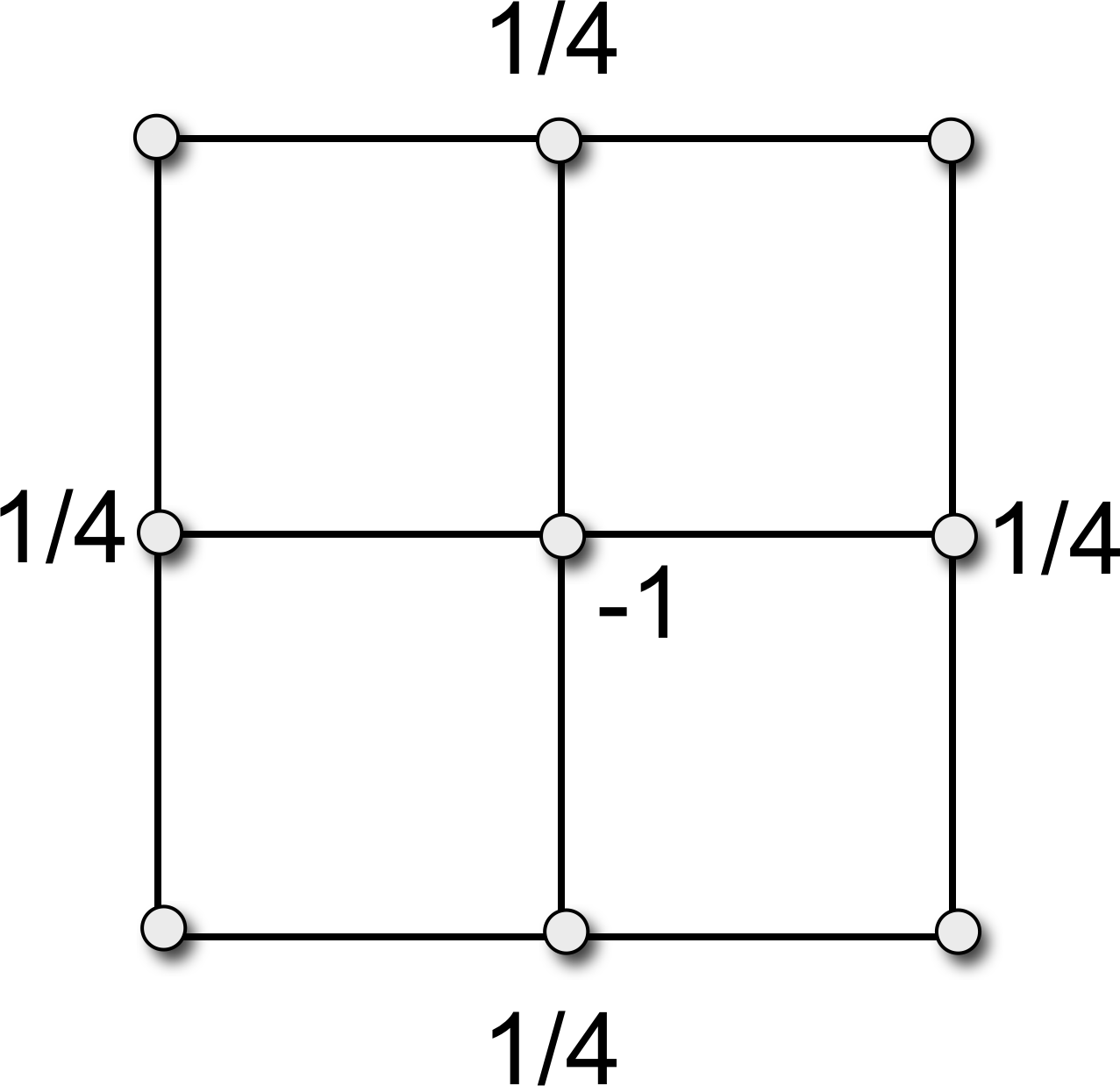
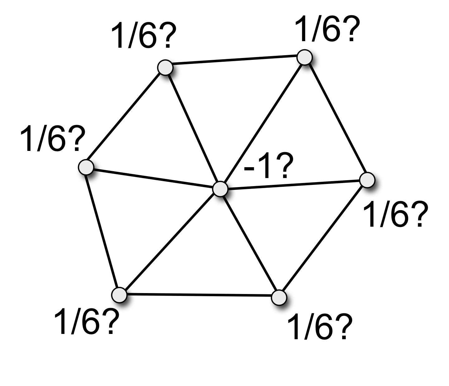
Uniform Laplace
- Uniform Laplace-Beltrami discretization \[ \laplace_\func{uni} f\of{v_i} \;:=\; \frac{1}{\abs{\set{N}_1\of{v_i}}} \sum_{v_j \in \set{N}_1\of{v_i}} \left( f\of{v_j} - f\of{v_i} \right) \]
- Properties
- simple and efficient
- depends only on connectivity
- does not take into account geometry at all
Uniform Laplace
- Uniform Laplace-Beltrami discretization \[ \laplace_\func{uni} \vec{x}_i \;:=\; \frac{1}{\abs{\set{N}_1\of{v_i}}} \sum_{v_j \in \set{N}_1\of{v_i}} \left( \vec{x}_j - \vec{x}_i \right) \;\approx\; -2 H \vec{n} \]
- Properties
- simple and efficient
- bad approximation for irregular triangulations, e.g. can give non-zero \(H\) for planar meshes
- does not take into account scale
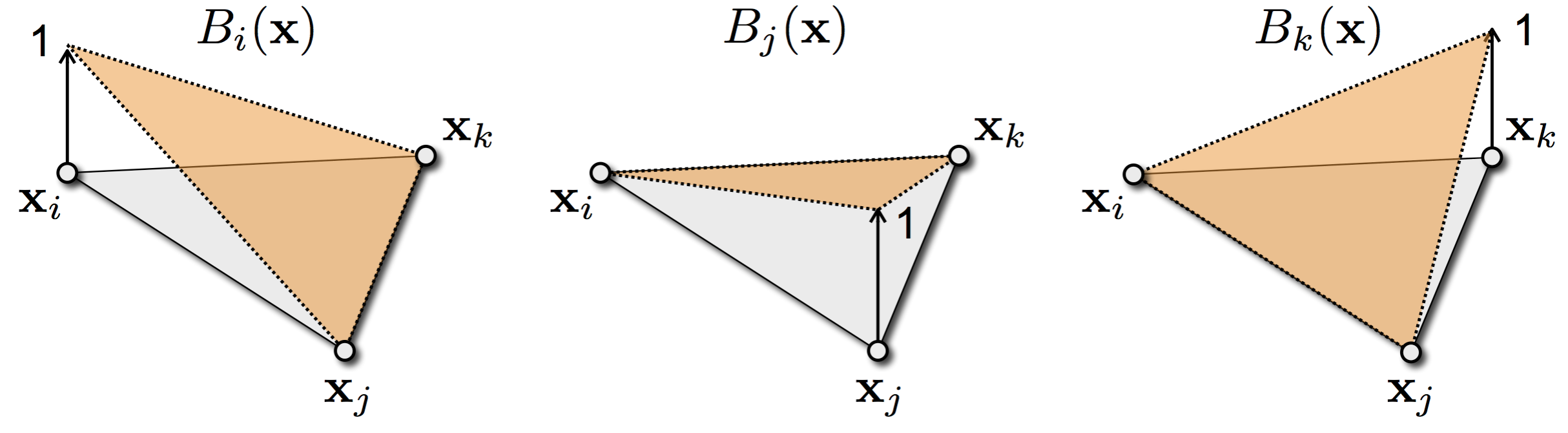
Functions on a Mesh
- Given per-vertex values \(f(v_i) = f(\vec{x}_i) = f(\vec{u}_i) = f_i\) we obtain a piecewise linear function per triangle
\[f(\vec{u}) \;=\; f_i B_i (\vec{u}) + f_j B_j(\vec{u}) + f_k B_k(\vec{u})\]
- We use linear basis functions \(B_i\), \(B_j\), \(B_k\) on a triangle
Gradients on a Mesh
- The gradient of the linear basis functions \(B_i\), \(B_j\), \(B_k\) is \[ \grad B_i (\vec{u}) \;=\;
\frac{ \left( \vec{x}_k - \vec{x}_j \right)^{\perp} }{ 2 \, A_T }
\,,\quad
\grad B_j (\vec{u}) \;=\;
\frac{ \left( \vec{x}_i - \vec{x}_k \right)^{\perp} }{ 2 \, A_T }
\,,\quad
\grad B_k (\vec{u}) \;=\;
\frac{ \left( \vec{x}_j - \vec{x}_i \right)^{\perp} }{ 2 \, A_T }
\]
- Combining with equations from previous slide we get \[ \grad f(\vec{u}) \;=\; \left( f_j - f_i \right) \frac{ \left( \vec{x}_i - \vec{x}_k \right)^{\perp} }{ 2 \, A_T } + \left( f_k - f_i \right) \frac{ \left( \vec{x}_j - \vec{x}_i \right)^{\perp} }{ 2 \, A_T } \]
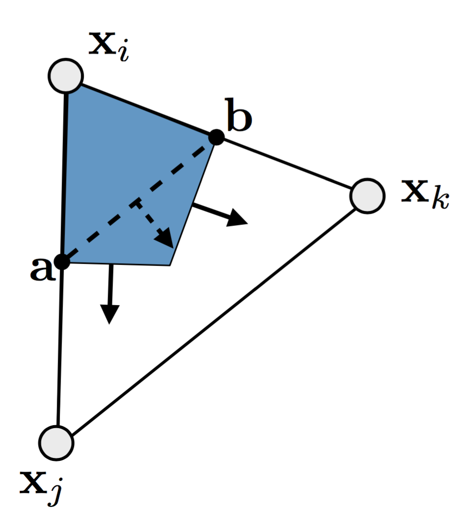
Divergence Theorem & Laplace
- Laplace operator \[ \int_{A_i} \Delta f(\vec{u}) \,\mathrm{d}A \;=\; \int_{\partial A_i} \grad f(\vec{u}) \cdot \vec{n}(\vec{u}) \,\mathrm{d}s \]
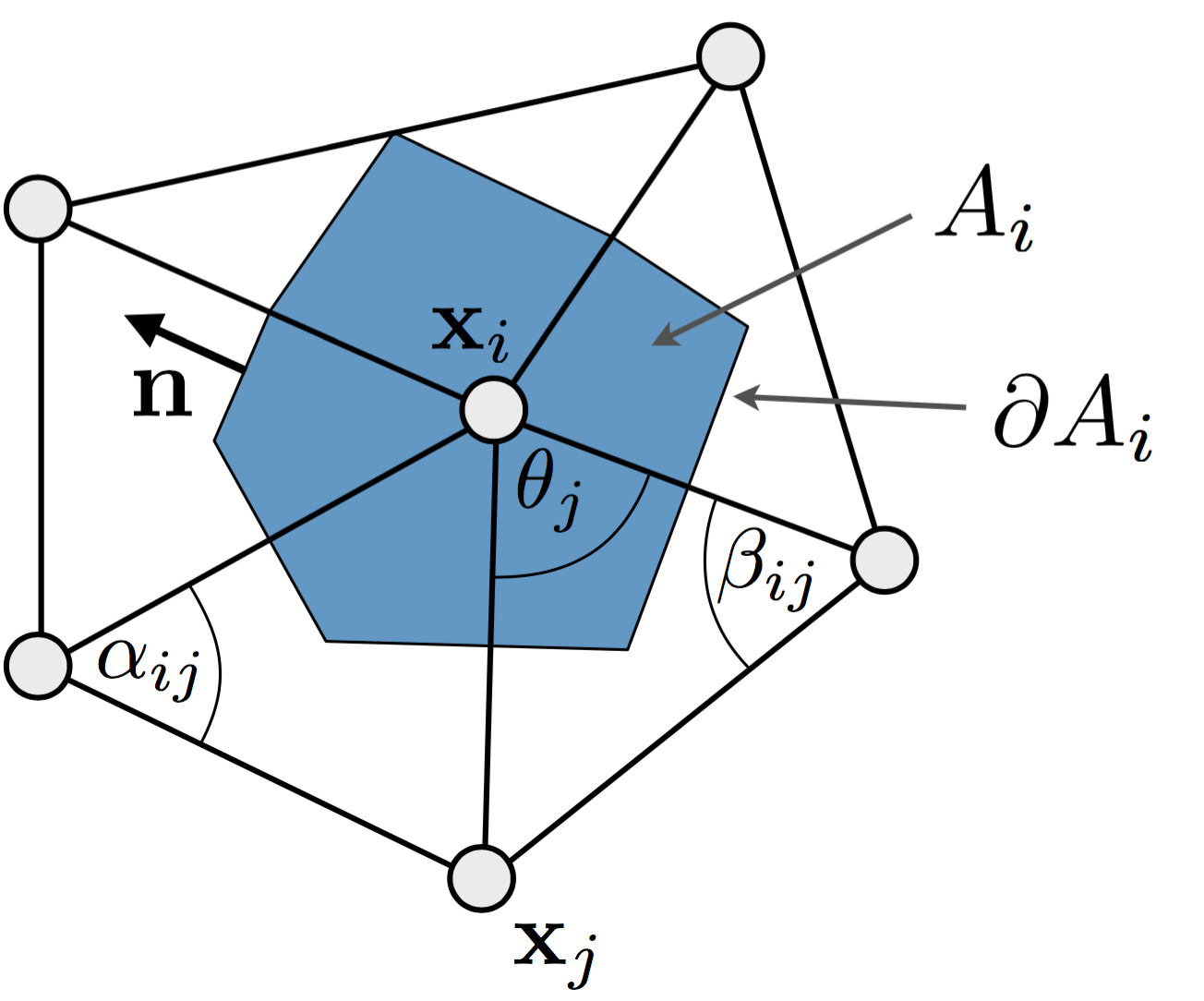
- Per triangle segment \[ \begin{align} \int_{\partial A_i \cap T} \grad f(\vec{u}) \cdot \vec{n}(\vec{u}) \mathrm{d}s & \;=\; \grad f(\vec{u}) \cdot (\vec{a} - \vec{b})^{\perp} \\ & \;=\; \frac{1}{2} \grad f(\vec{u}) \cdot (\vec{x}_j - \vec{x}_k)^{\perp} \end{align} \]
Discrete Laplace-Beltrami
\[ \begin{align*} \int_{\partial A_i \cap T} \grad f(\vec{u}) \cdot \vec{n}(\vec{u}) \mathrm{d}s & \;=\; \frac{1}{2} \grad f(\vec{u}) \cdot (\vec{x}_j - \vec{x}_k)^{\perp} \\ & \;=\; \begin{split}\left(f_j-f_i \right) \frac{\left(\vec{x}_i-\vec{x}_k \right)^{\perp} \cdot \left(\vec{x}_j-\vec{x}_k \right)^{\perp}}{4 A_T} \\ \;+\; \left(f_k-f_i \right) \frac{\left(\vec{x}_j-\vec{x}_i \right)^{\perp} \cdot \left(\vec{x}_j-\vec{x}_k \right)^{\perp}}{4 A_T}\end{split}\\ & \;\;\vdots\; \\ & \;=\; \frac{1}{2} \cot \gamma_k \left(f_j - f_i \right) \;+\; \frac{1}{2} \cot \gamma_j \left(f_k - f_i \right) \end{align*} \]
Discrete Laplace-Beltrami
- Cotangent discretization
\[ \laplace_{\set{S}} f\of{v_i} \;:=\; \frac{1}{2A\of{v_i}} \sum_{v_j \in \set{N}_1\of{v_i}} \left( \cot \alpha_{ij} + \cot \beta_{ij} \right) \left( f\of{v_j} - f\of{v_i} \right)\]
Literature
- Botsch et al., Polygon Mesh Processing, AK Peters, 2010
- Chapter 3
- Meyer et al.: Discrete Differential-Geometry Operators for Triangulated 2-Manifolds. In Visualization and Mathematics III, Springer, 2003.