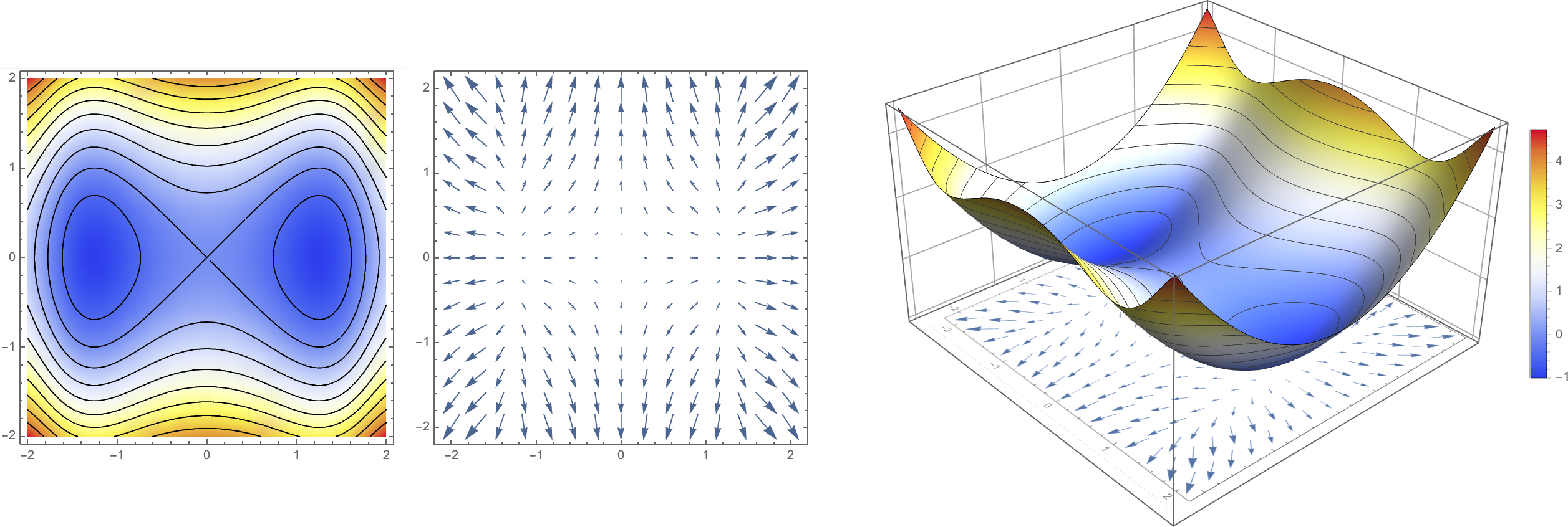
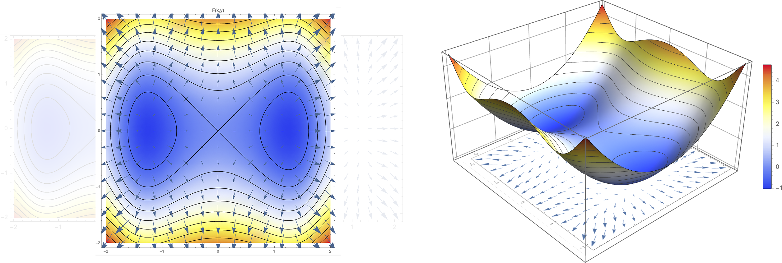
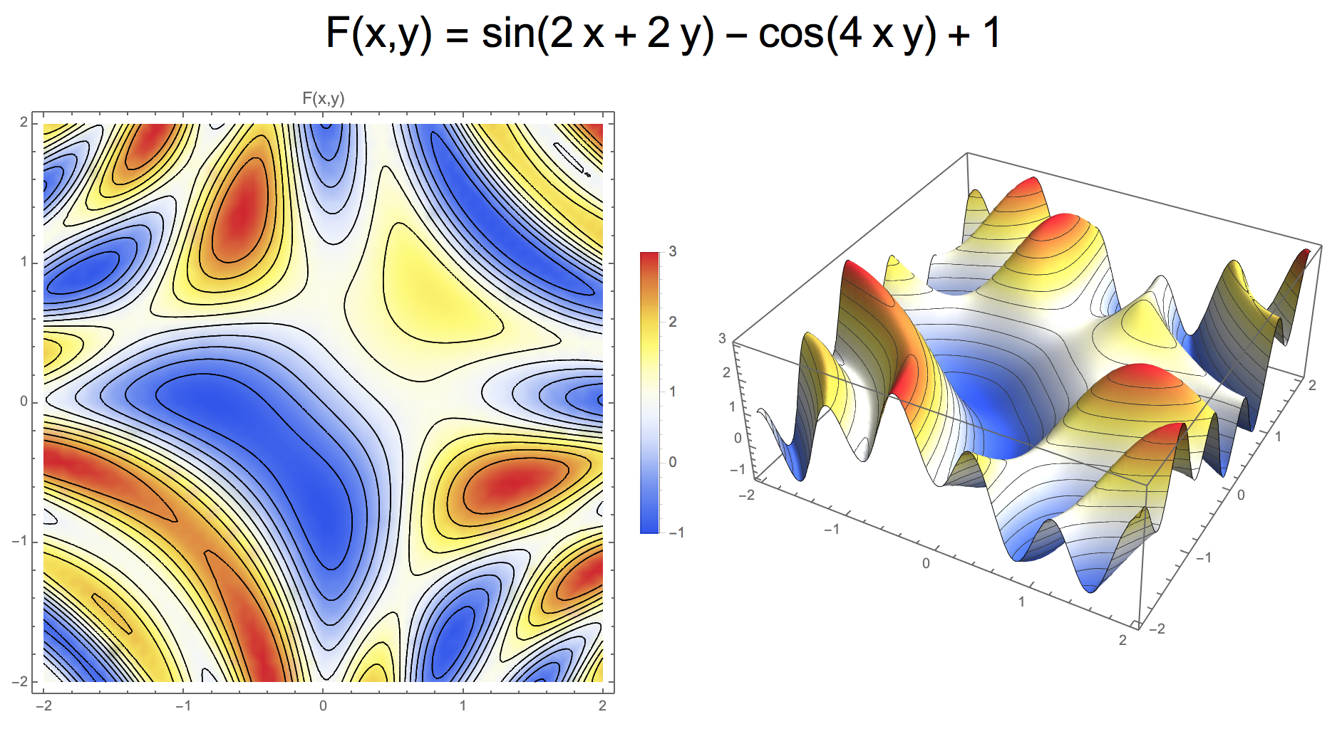
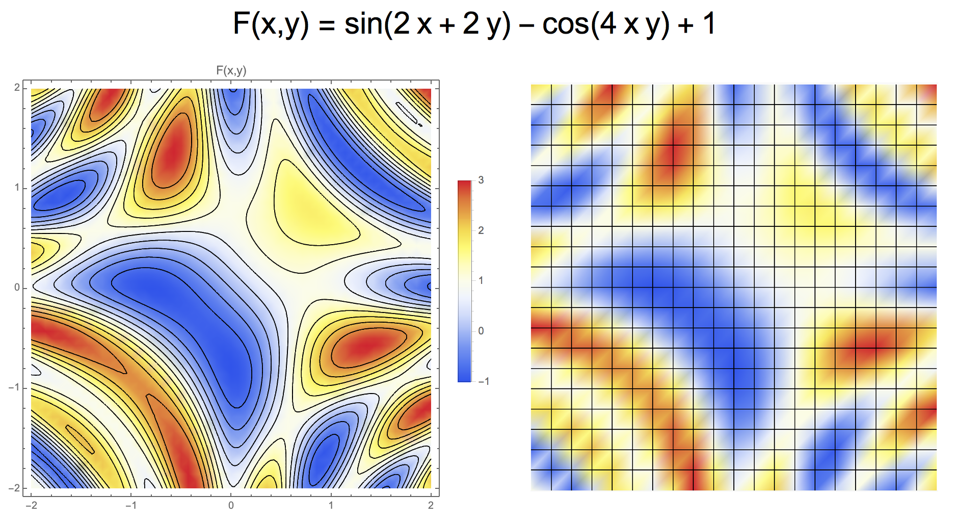
Gradient of function \(F : \R^n \mapsto \R\) is defined as \[\nabla F = \left[ \frac{\partial F}{\partial x_1} \; \frac{\partial F}{\partial x_2} \; \cdots \;\frac{\partial F}{\partial x_n} \right]^T\]
\(\nabla F\) points into the direction of steepest ascent. Why?
Gradient of function \(F : \R^n \mapsto \R\) is defined as \[\nabla F = \left[ \frac{\partial F}{\partial x_1} \; \frac{\partial F}{\partial x_2} \; \cdots \;\frac{\partial F}{\partial x_n} \right]^T\]
Gradient \(\nabla F\) is orthogonal to level set
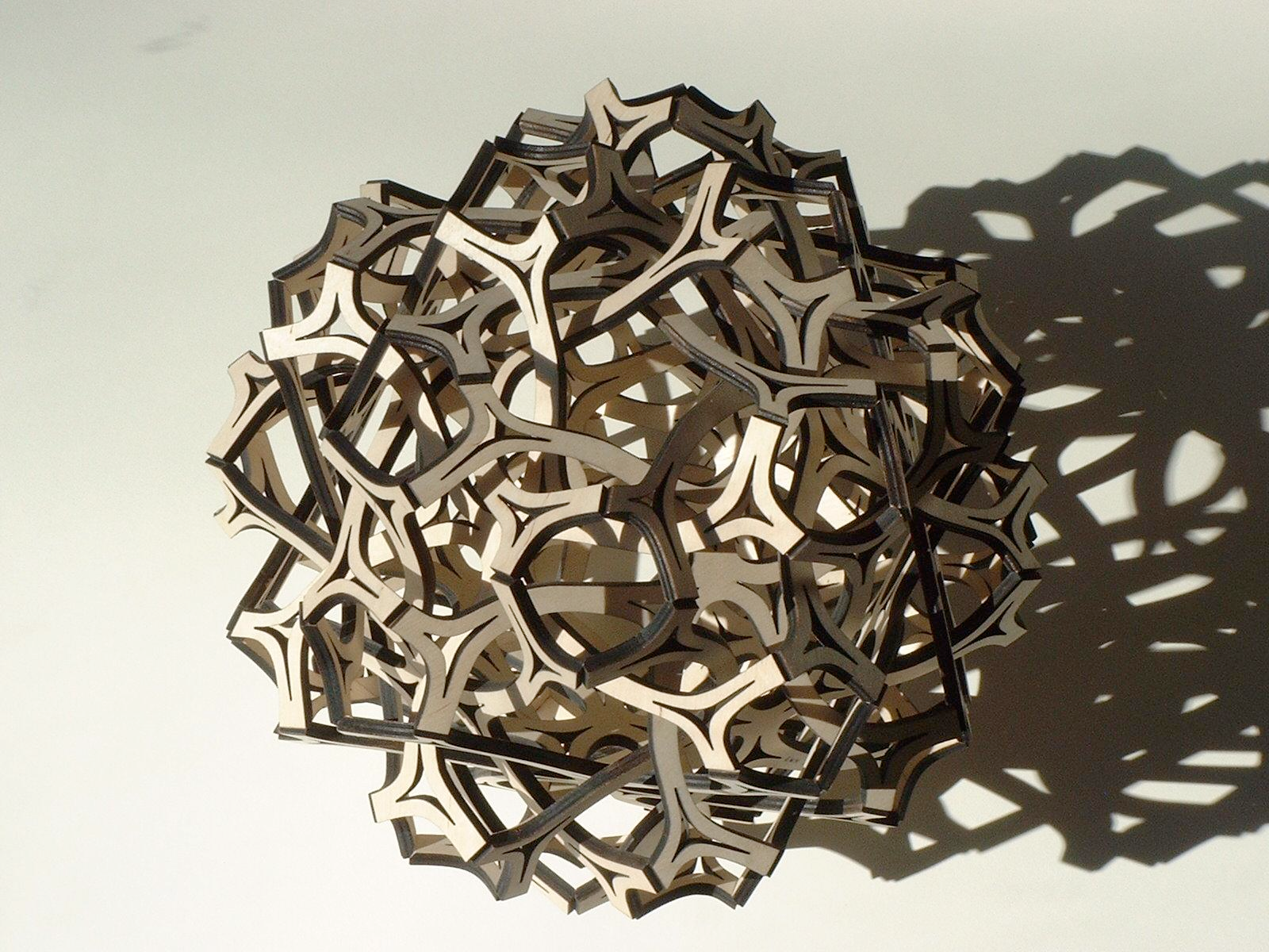
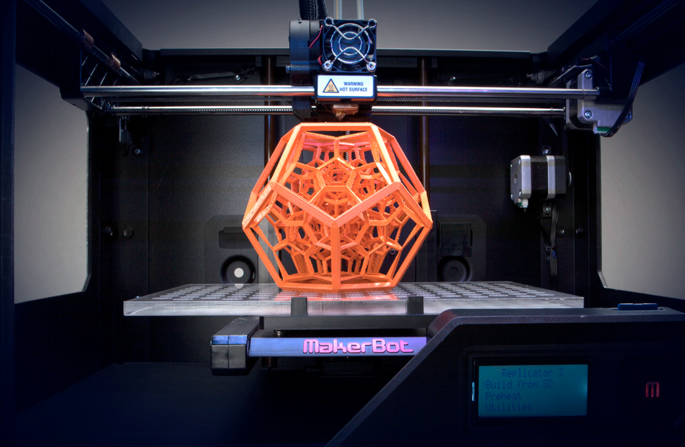
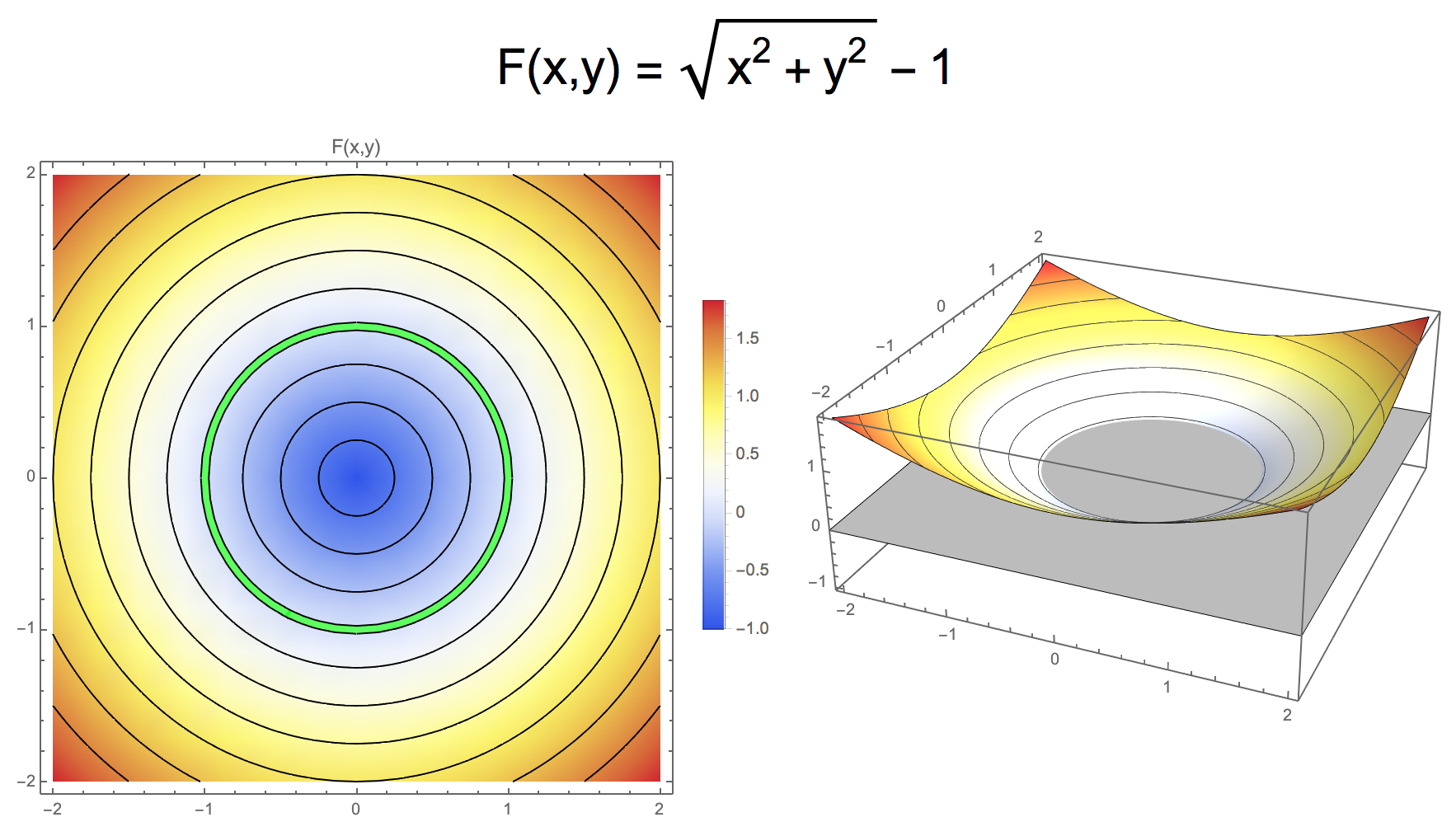
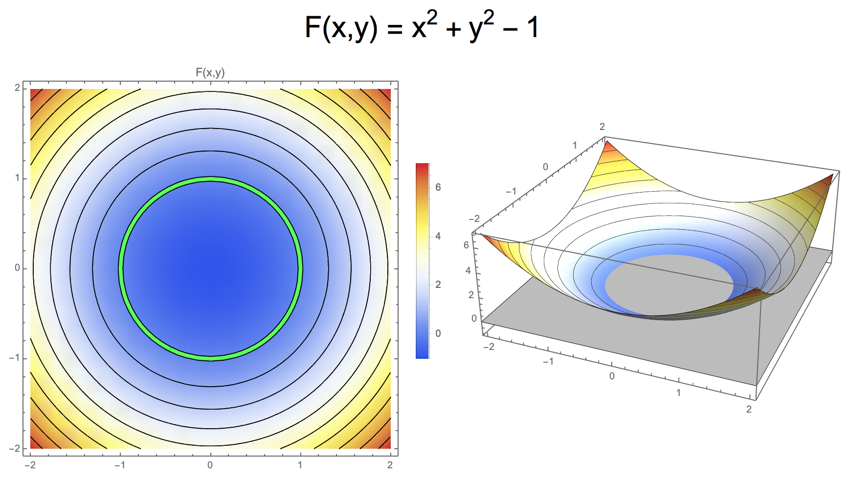
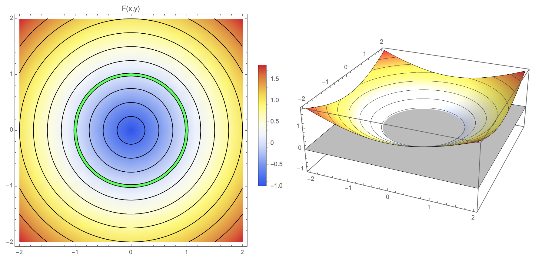
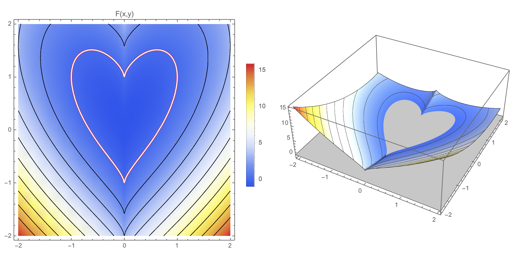
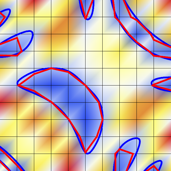
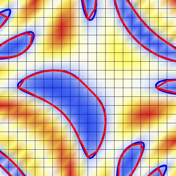
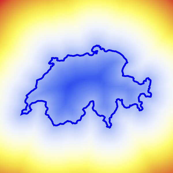
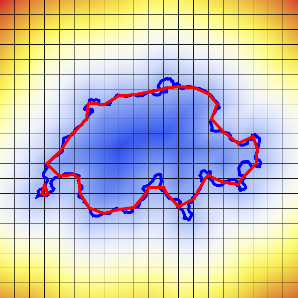
Signed Distance Function (SDF)
Special case of an implicit representation
\(F(\vec{x})\) gives signed distance to closest point on level surface
simple: \(\vec{x}\of{t}\) is injective (no self-intersections)
differentiable: \(\vec{x}’\of{t}\) is defined for all \(t \in [a,b]\)
regular: \(\vec{x}’\of{t} \neq \vec{0}\) for all \(t \in [a,b]\)
Which of the following are simple, differentiable, regular?
Re-parameterization
We can represent the same geometry with different parameter functions
For example, the same curve is defined for \(t \in [0,1]\) by the functions \[\vec{x}_1\of{t} = \matrix{\sin(4 \pi t) \\ \cos(2 \pi t)}
\;\text{ and }\;
\vec{x}_2\of{t} = \matrix{\sin(4 \pi \sqrt{t}) \\ \cos(2 \pi \sqrt{t})}\]
In other words, the image of \([0,1]\) under \(\vec{x}_1\) and \(\vec{x}_2\) is equivalent
We can map from \(\vec{x}_1\) to \(\vec{x}_2\) using a re-parameterization function \(u\)
In our example, we have \(u \colon [0,1] \to [0,1]\) with \(u(t) = \sqrt{t}\)
If \(\vec{x}_1(t) = \vec{c}(t)\), then \(\vec{x}_2(t) = \vec{c}(u(t))\)
Re-parameterization
We can map from \(\vec{x}_1\) to \(\vec{x}_2\) using a re-parameterization function \(u\)
In our example, we have \(u \colon [0,1] \to [0,1]\) with \(u(t) = \sqrt{t}\)
If \(\vec{x}_1(t) = \vec{c}(t)\), then \(\vec{x}_2(t) = \vec{c}(u(t))\)
Parameter intervals do not need to be identical!
For example, if \(\vec{x}_1 \colon [a,b] \to \R^2\) and \(\vec{x}_2 \colon [c,d] \to \R^2\) define the same curve, we can define a re-parameterization function \(u \colon [a,b] \to [c,d]\) such that \(\vec{x}_1(t) = \vec{x}_2(u(t))\)
Quiz
Which of the following parametric curves have the same geometry as \(\trans{[ \cos(t), \sin(t)]}, t \in [0, \pi]\)?
\(\matrix{\cos(2t) \\ \sin(2t)} ,\; t \in [ 0, 2\pi]\)
\(\matrix{t \\ \sqrt{1-t^2} } ,\; t \in [-1, 1 ]\)
\(\matrix{\cos(t^2) \\ \sin(t^2)} ,\; t \in [0, \pi ]\)
\(\matrix{\sin(t) \\ -\cos(-t)} ,\; t \in [\frac{\pi}{2}, \frac{3\pi}{2}]\)
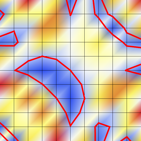
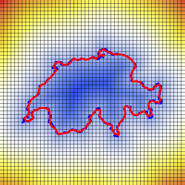
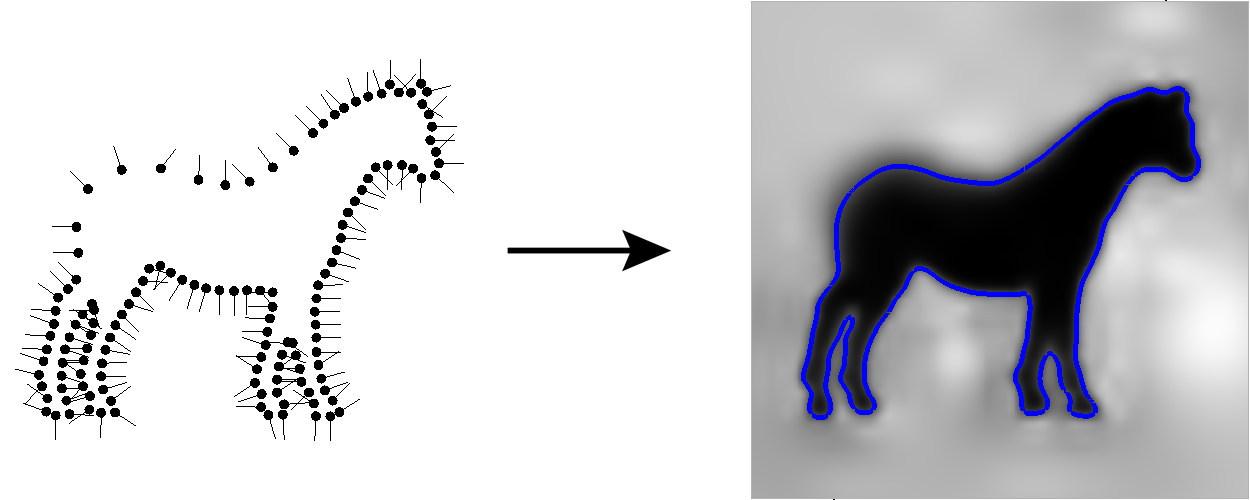
Discrete Explicit Representation
Sample the parameter interval \([a,b]\), e.g., at parameters \(t_i = a + i \frac{b-a}{n},\; i = 0, \ldots, n\)
Then the polyline through the points \(\vec{x}\of{t_i}\) is a piecewise linear approximation of the curve \(\vec{x}\)
With increasing \(n\), the polyline converges to the curve
Length of a Curve
How can we measure length of a continuous curve?
Example: What is the length of a parabola \(y = x^2\), \(x \in [0,1]\)?
We know how to measure the length of a polyline!
Let \(t_i = a + i \Delta t\) and \(\vec{x}_i = \vec{x}\of{t_i}\)