Computer Graphics
Outro
Computer Graphics
Group


Basic Ray Tracing Pipeline
- Implementing a ray tracer basically comes down to three operators that we have to understand and implement.


Ray-Triangle Intersection (explicit)
- Ray and triangle have to coincide \[ \vec{o} + t\,\vec{d} \;=\; \alpha\vec{A} + \beta\vec{B} + \gamma\vec{C}\] Four unknowns, but only three equations!
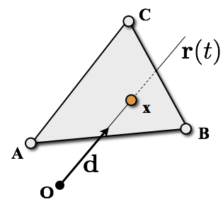
- Exploit condition \(\alpha+\beta+\gamma=1\) to eleminate \(\alpha\) \[ \vec{o} + t\,\vec{d} \;=\; (1-\beta-\gamma)\vec{A} + \beta\vec{B} + \gamma\vec{C}\] Solve \(3 \times 3\) linear system (Cramer’s rule)
- Check inside conditions: \(0 \leq \alpha, \beta, \gamma \leq 1\)
Lighting

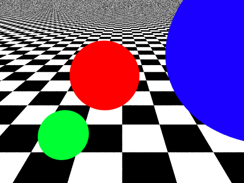 no illumination
 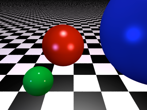 local illumination
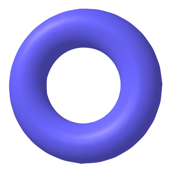
 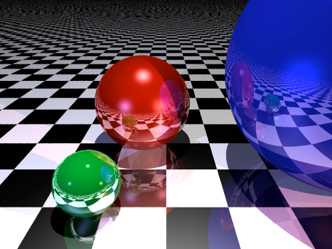 global illumination
Phong Lighting Model
 ambient: \(I_a m_a\)
 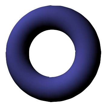 diffuse: \(I_l m_d \left( \vec{n} \cdot \vec{l} \right)\)
 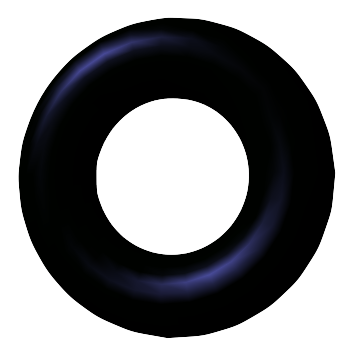 specular: \(I_l m_s \left( \vec{r} \cdot \vec{v} \right)^s\)
 \[
I \;=\;
I_a m_a +
I_l \left(
m_d \left( \vec{n} \cdot \vec{l} \right) +
m_s \left( \vec{r} \cdot \vec{v} \right)^s
\right)
\]
\[
I \;=\;
I_a m_a +
I_l \left(
m_d \left( \vec{n} \cdot \vec{l} \right) +
m_s \left( \vec{r} \cdot \vec{v} \right)^s
\right)
\]
Shadows
- Send shadow ray from intersection point to light source.
- Discard diffuse and specular contribution if light source is blocked by another object.


Recursive Ray Tracing
At each intersection point, reflect and/or refract incoming viewing ray at surface normal, and trace child rays recursively.
The final color is interpolated between local illumination, reflection, and refraction based on material properties.
Limits of Raytracing
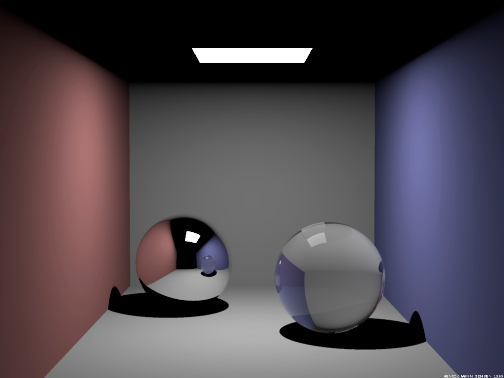 standard ray tracing
 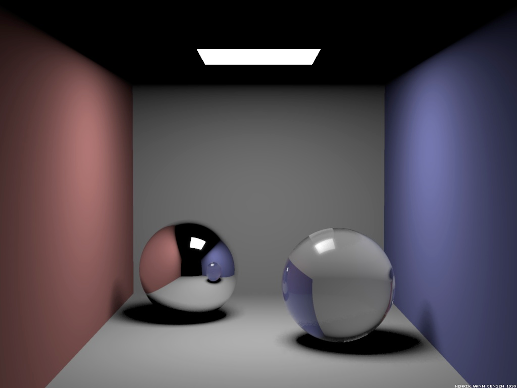 +soft shadows
 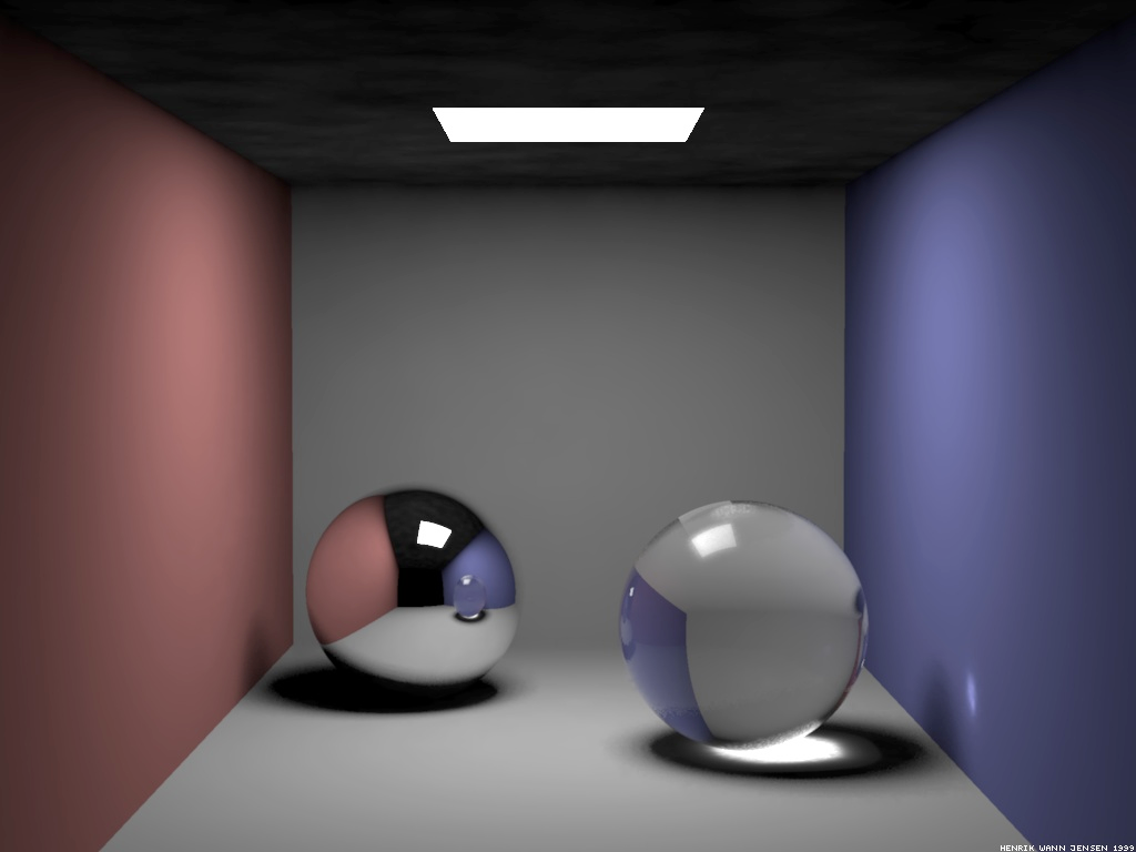 +caustics
 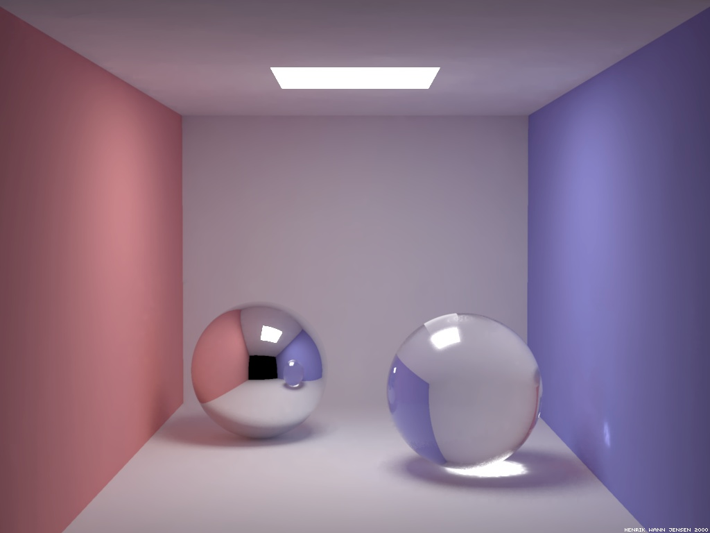 +indirect lighting
Light Paths

- E = eye point
- L = light source
- D = diffuse reflection
- S = specular reflection
Ray Tracing vs. Rasterization
- Ray Tracing
- Shoot rays from 2D pixels into 3D scene
- “backward rendering”
- needs ray intersections

- Rasterization
- Project 3D objects onto 2D image plane
- “forward rendering”
- needs transformations, projections, visibility computation

Rasterization Pipeline

Transformations & Projections

 scaling
  rotation
  translation
Transformations & Projections
- Linear and affine transformations
- Homogenous coordinates
- Matrix representation
Transformations & Projections
Transformations & Projections
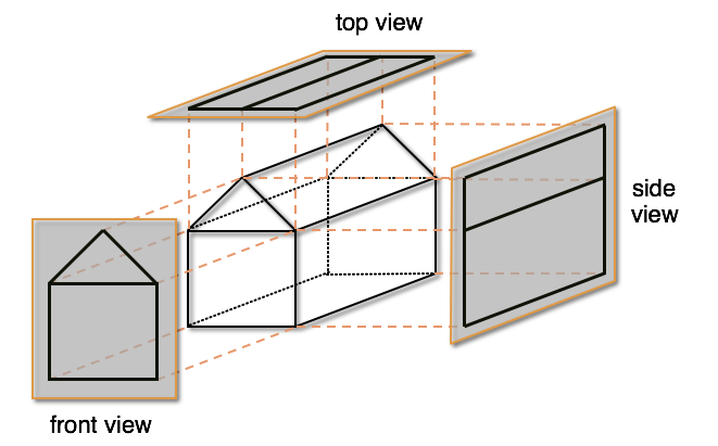
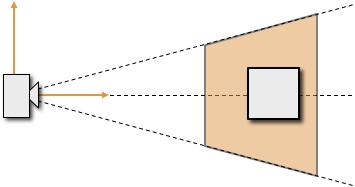
- Types of projections
- Derivation of perspective projections
- Coordinate systems and matrix representation
Lighting

ambient 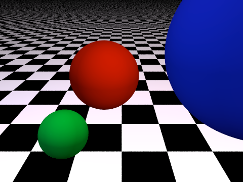 +diffuse +specular
Clipping


Rasterization

Rasterization
- Bresenham Algorithm
- implicit vs explicit representation
- integer arithmetic
Shading

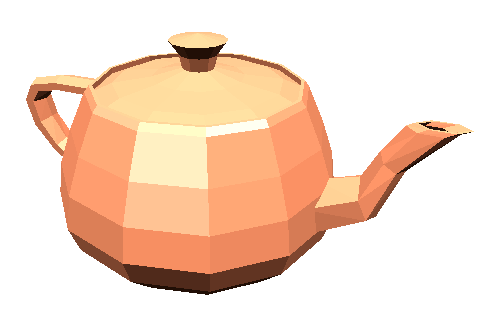 flat
flat 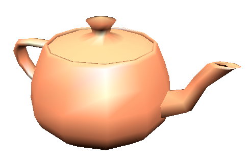 Gouraud
 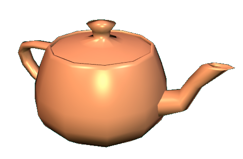 Phong
Phong
Visibility

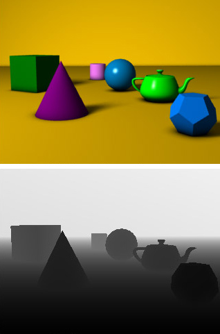

Visibility
- Painters algorithm vs. z-buffer
- Potential issues of z-buffer
Forward Problem
- Which L-System rule produces the following output given axiom F at level 5 and angle 90?
- \(F \rightarrow F-F+F\)
- \(F \rightarrow F+FF\)
- \(F \rightarrow FFF+FF\)
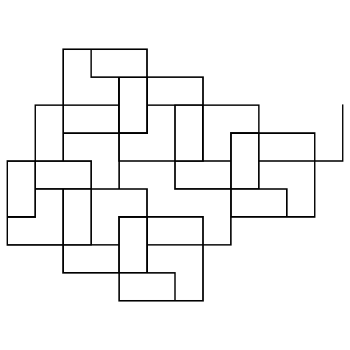
Inverse Problem
- Which L-System creates this output?
- define the axiom and the rule(s)
 level 0 = axiom
  level 1
  level 2
  level 3