Computer Graphics
Bézier Curves I


Course Evaluation
- Feedback possible till December 15th, 18:00
- Please participate
- Add additional comments
- Link

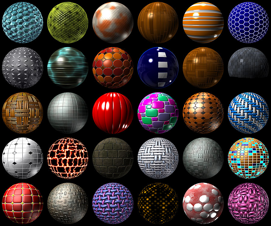
Procedural Techniques
- Ubiquitous in graphics
- texturing, modeling, animation, etc.

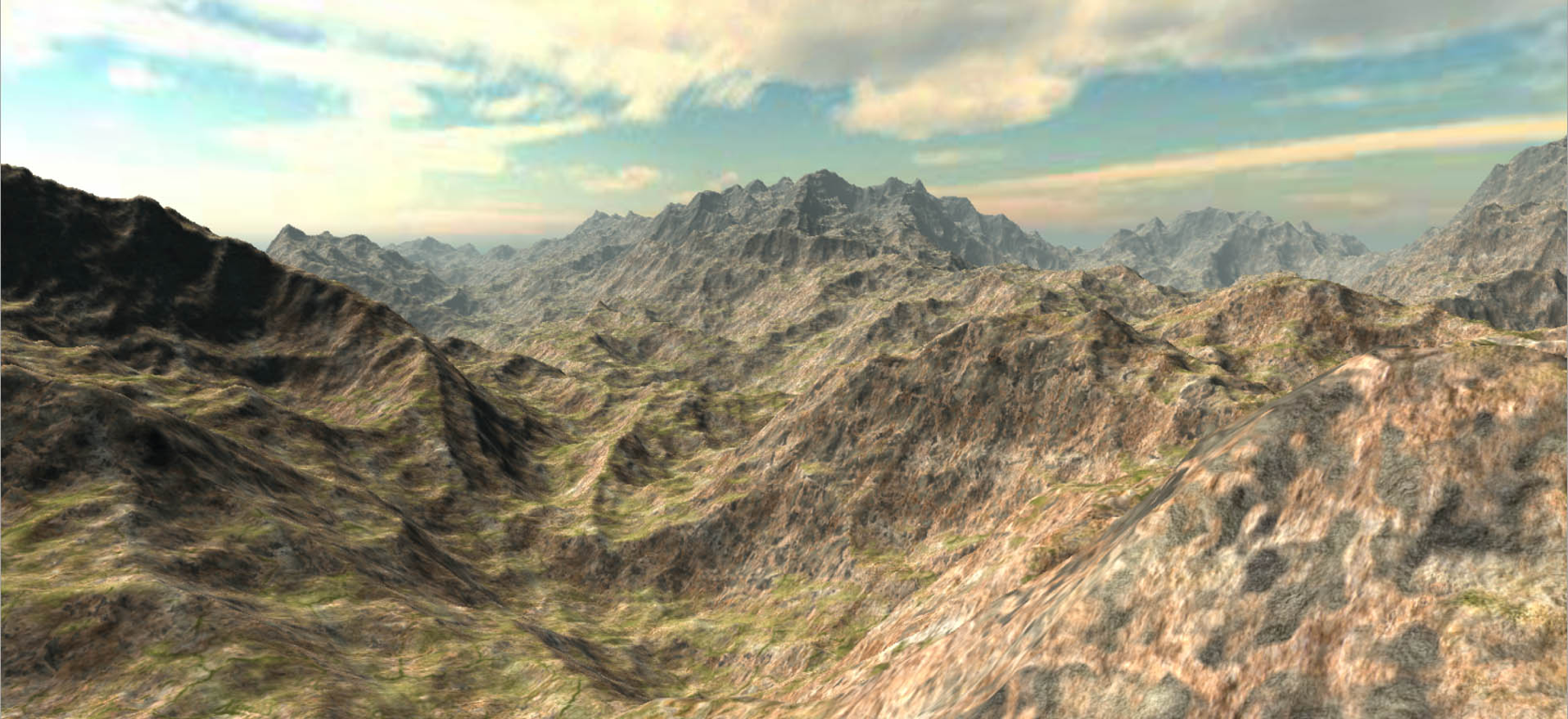
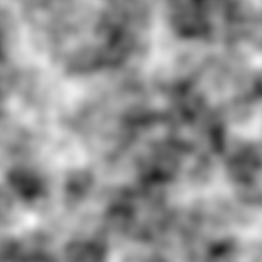
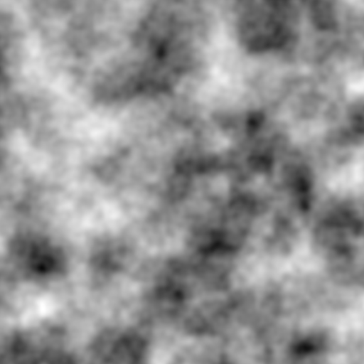
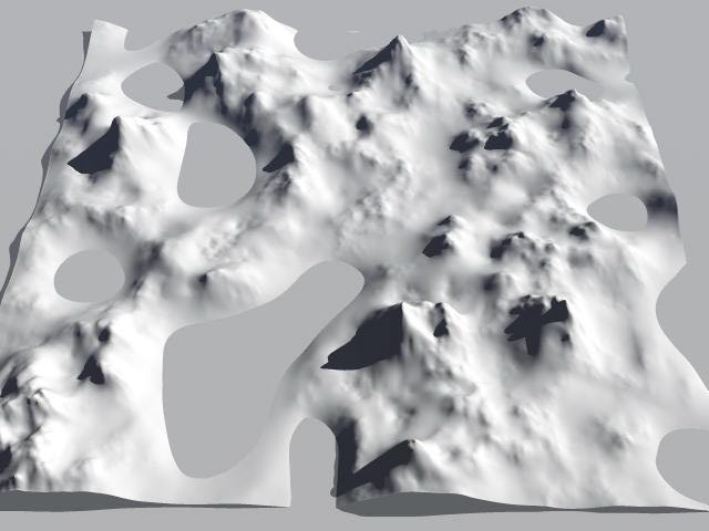
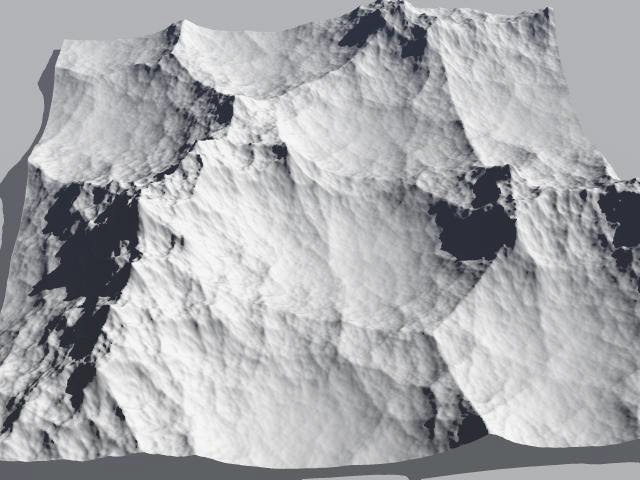
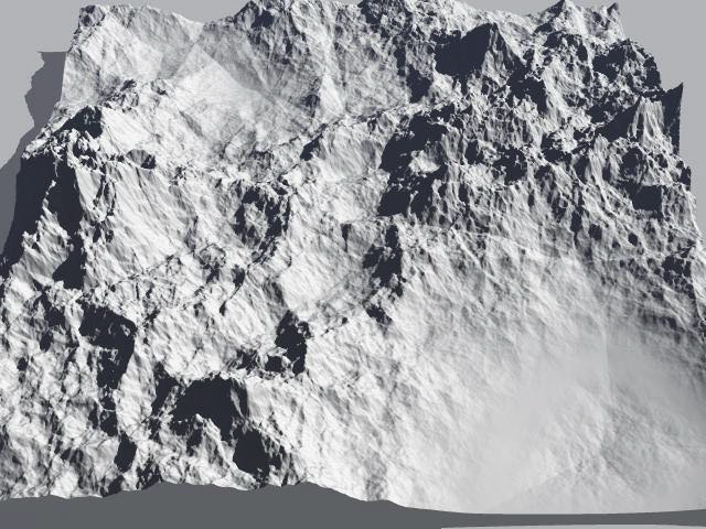
Fractal Brownian Motion (fBm)
- Spectral synthesis of noise function
- Progressively smaller frequency
- Progressively smaller amplitude
- Typically Perlin noise is used
- Each term in the summation is called an octave
- Each octave typically doubles frequency and halves amplitude

Fractal Dimension Example: Koch Curve

\[ \begin{aligned} D &= \frac{\log(N)}{\log(r)} \\ \end{aligned} \]
\[ \begin{aligned} \\ N &= 4 \\ r &= 3 \\ D &= \log(4)/\log(3) \\ &= 1.26185951... \end{aligned} \]
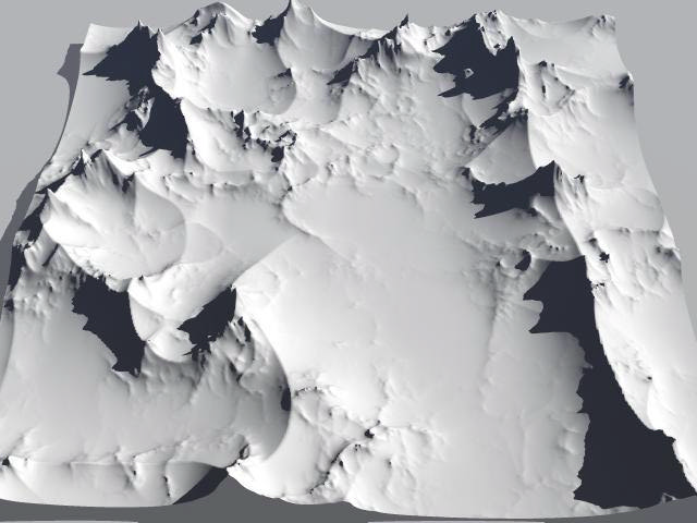
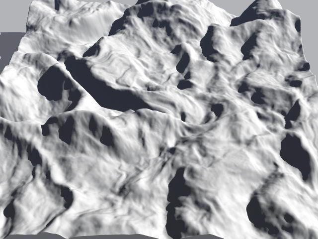
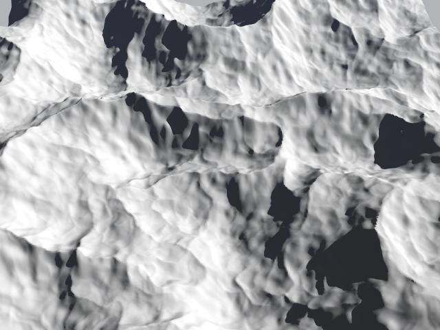
Heterogeneous fBm
Overview

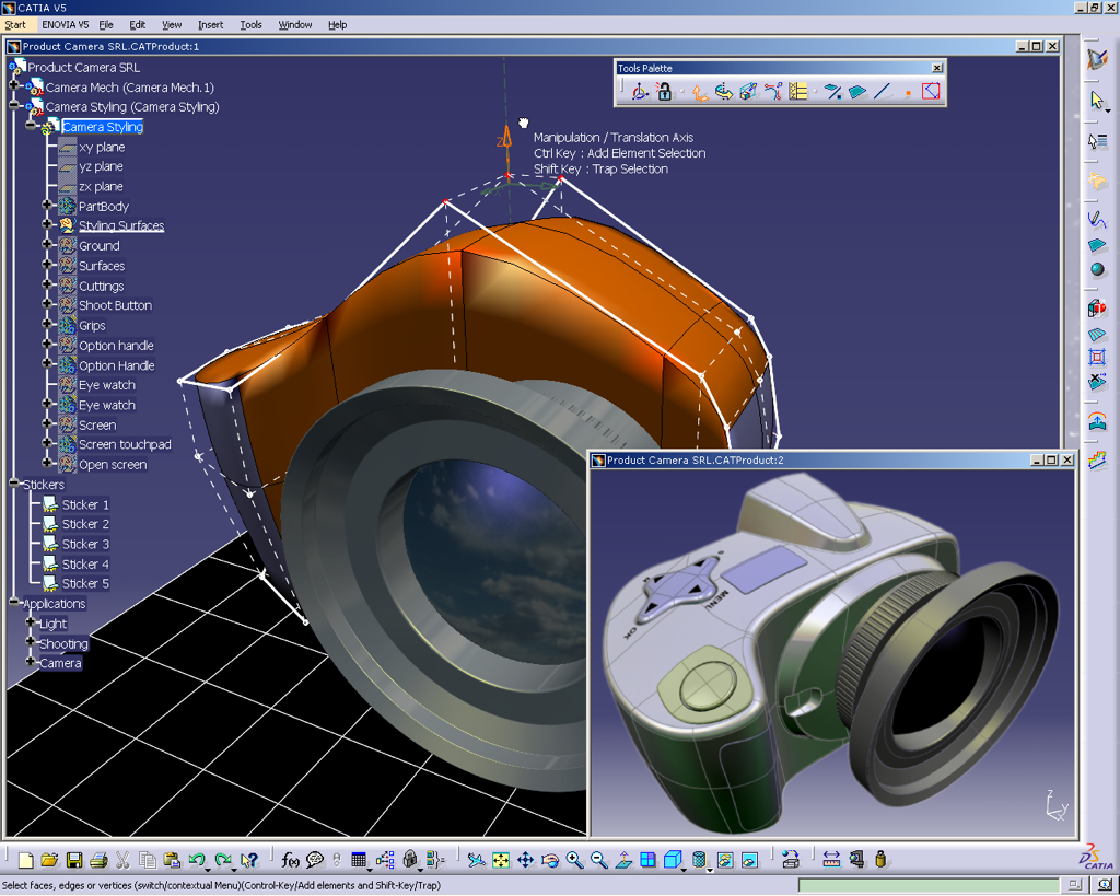
Example: Dassault’s CATIA
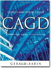
Literature
- Farin: Curves and Surfaces for CAGD. A Practical Guide, Morgan Kaufmann, 2001
- Chapters 4 & 5
How to make LOVE?
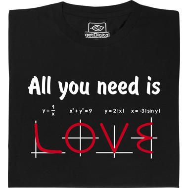

Guess the shape of the curve!
\[\vec{x}\of{t} = \matrix{\sin^3(t) \\ \frac{1}{16}(13\cos(t) - 5 \cos(2t) - 2 \cos(3t)-\cos(4t))}\]


Discrete Curves
- Approximate the curve by a polygon, e.g. for rendering
- Sample parameter interval: \(t_i = a + i\Delta t\)
- Sample curve: \(\textbf{x}_i = \textbf{x}(t_i)\)
- Connect samples by polygon


Polynomial Curves
\[ \vec{x}(t) = \sum_{i=0}^n \vec{b}_i \, \phi_i(t) \;\in \Pi^n\]
- Ingredients
- Vector-valued coefficients \(\vec{b}_i \in \R^3\)
- Scalar-valued polynomials \(\phi_i \colon \R \rightarrow \R\)
- \(\{ \phi_0, \ldots, \phi_n \}\) span space of degree \(n\) polynomials
- Why polynomials?
- Can be computed efficiently on a computer (only multiplications and additions needed)
- Can approximate arbitrary functions (Weierstrass approximation theorem)
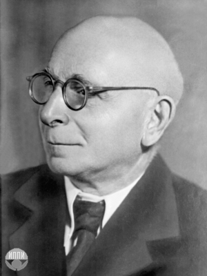
1815-1897
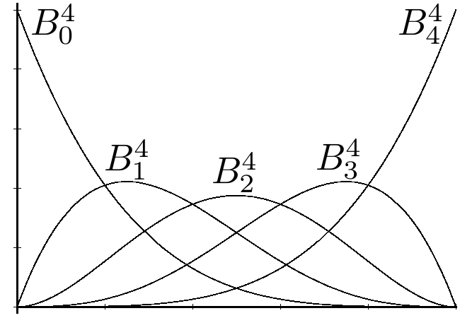
Bernstein Polynomials
\[ \begin{align*} B_i^n(t) &\;=\; \binom{n}{i} t^i (1-t)^{n-i} \,,\quad 0 \leq i \leq n\\ \binom{n}{i} &\;=\; \begin{cases} \frac{n!}{i!(n-i)!} & \text{if }0 \leq i \leq n, \\ 0 & \text{otherwise.} \end{cases} \end{align*} \]
1880-1968
Bernstein Polynomials
\[B_i^n(t) = \binom{n}{i} t^i (1-t)^{n-i}\]
- Basis: \(\{ B_0^n, \ldots, B_n^n \}\) are a basis for \(\Pi^n\)
- Non-negativity: \(B_i^n(t) \geq 0\) for \(t \in [0,1]\)
- Endpoints: \(B_i^n(0) = \delta_{i,0}\) and \(B_i^n(1) = \delta_{i,n}\)
- Symmetry: \(B_i^n(t) = B_{n-i}^n(1-t)\)
- Maximum: \(B_i^n(t)\) has maximum at \(t=i/n\).
- Partition of unity: \(\sum_{i=0}^n B_i^n(t) = 1\)
Bezier Curves
Bezier curves use Bernstein polynomials as basis: \[\vec{x}(t) = \sum_{i=0}^n \vec{b}_i \, B_i^n(t)\]
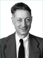
1910-1999
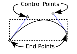
- Coefficients \(\vec{b}_i\) are called control points
- Points \(( \vec{b}_0, \ldots, \vec{b}_n )\) define the control polygon.
de Casteljau Algorithm
- Given:
- Control polygon \(\vec{b}_0,\ldots,\vec{b}_n\)
- Curve parameter \(t\)
- Initialization: \(\vec{b}_i^0 = \vec{b}_i \quad i=0, \ldots, n\)
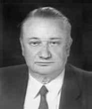
*1930
- Recursion: \[ \vec{b}_i^k = (1-t)\,\vec{b}_i^{k-1} + t\,\vec{b}_{i+1}^{k-1} \] where \(k = 1,\ldots,n\) and \(i = 0,\ldots,n-k\)
- Result: \(\vec{b}_0^n = \sum_{i=0}^n \vec{b}_i B_i^n(t) = \vec{x}(t)\)

Geometric Interpretation
de Casteljau Construction
\[\begin{eqnarray*} \sum_{i=0}^n \vec{b}_i B_i^n(t) &=& \sum_{i=0}^n \vec{b}_i \left[ (1-t)\,B_i^{n-1}(t) \;+\; t\,B_{i-1}^{n-1}(t) \right] \\ &=& \sum_{i=0}^{n-1} \left[ (1-t)\,\vec{b}_i \;+\; t\,\vec{b}_{i+1} \right] \, B_{i}^{n-1}(t) \end{eqnarray*}\]

Applications of Bezier Curves
Bezier curves are the most prominent curve representation:
- Used for 2D vector drawing applications
- Used for 3D computer-aided design (CAD)
- Used for true-type fonts
 Inkscape Dassault CATIA
 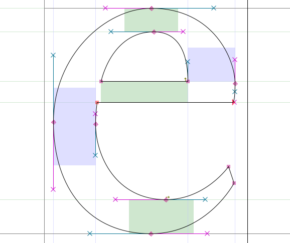 FontForge
Literature
- Farin: Curves and Surfaces for CAGD. A Practical Guide, Morgan Kaufmann, 2001
- Chapters 4 & 5