Computer Graphics
Texture & Shadows


Transformations & Projections

Lighting

Rasterization

Visibility

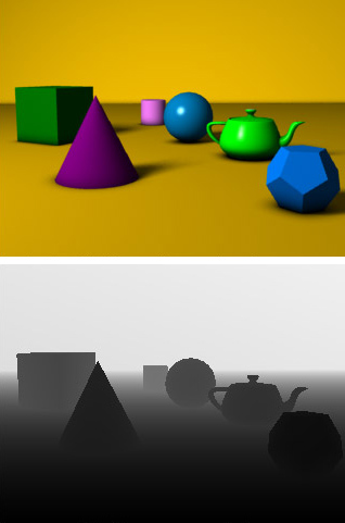
Z-Buffer
- Store current min. z-value for each pixel
- After model transformation, view transformation, projection transformation, and viewport transformation
- Additional buffer for depth values
- Framebuffer stores RBG color values
- Depth buffer (z-buffer) stores depth values
- Storage: additional 16 to 32 bits per pixel
Z-Buffer

Materials & Texture
So far: color/material varies per model or per vertex
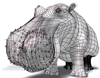
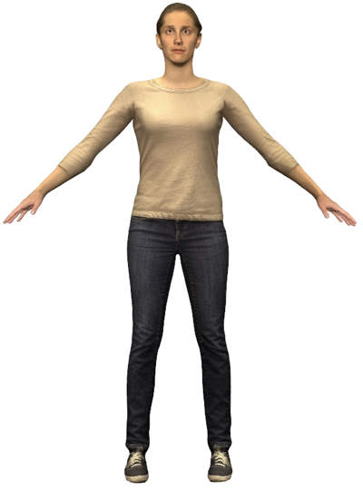
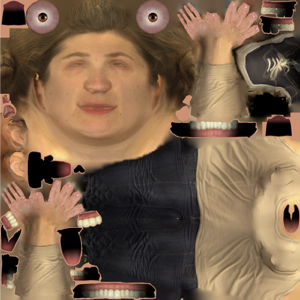
Textures add visual detail without raising geometric complexity: Paste 2D images onto 3D geometry
 Geometry
 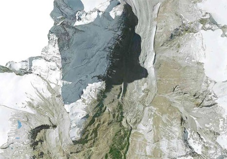 Texture
 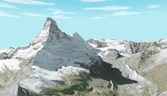 Textured Mesh
Materials & Texture
So far: color/material varies per model or per vertex
Textures add visual detail without raising geometric complexity: Paste 2D images onto 3D geometry
 Geometry
 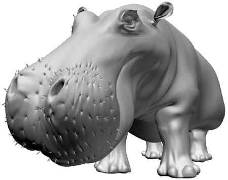 +Lighting
 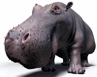 +Texture
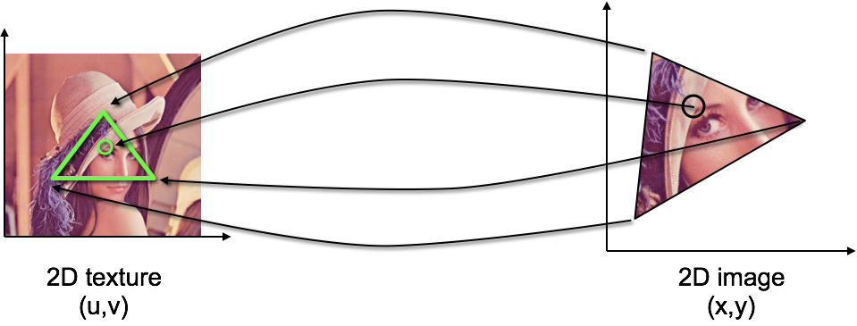
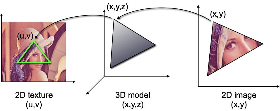
Texturing One Triangle
- Assign 2D texture coordinate \(\vec{u}=(u,v)\) to each vertex
- Interpolate texture coordinate by barycentric coordinates \[ \vec{u}\of{\vec{X}} = \alpha \vec{u}\of{\vec{A}} + \beta \vec{u}\of{\vec{B}} + \gamma \vec{u}\of{\vec{C}} \]
- Fetch color value from texture: \(\vec{c}\of{\vec{x}} = \mathrm{texture}\of{\vec{u}\of{\vec{x}}}\)
Texturing One Triangle
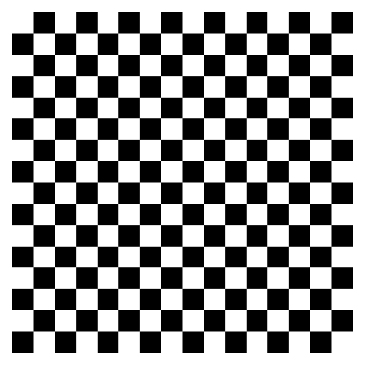
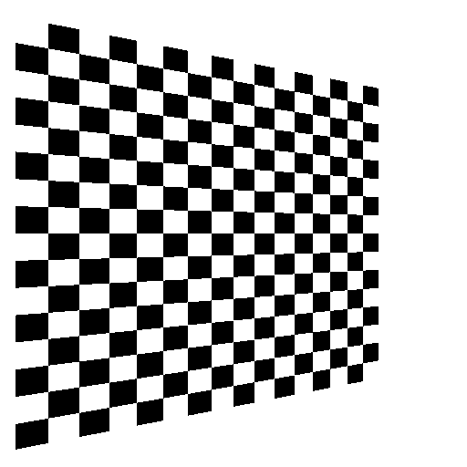
perspectively incorrect
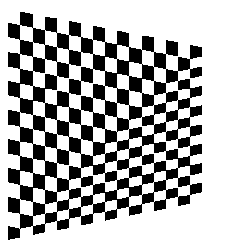
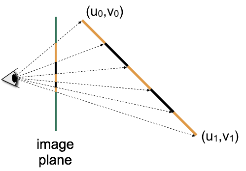
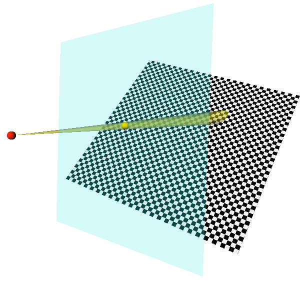
Perspective Interpolation
- Linear interpolation in world coordinates yields nonlinear interpolation in screen coordinates!
- Choose screen-space (
noperspective) or perspective (smooth) interpolation for vertex shader outputs (smoothis default)
Texturing One Triangle
- Assign 2D texture coordinate \(\vec{u}=(u,v)\) to each vertex
- Interpolate texture coordinate by barycentric coordinates in 3D object space
- Fetch color value from texture
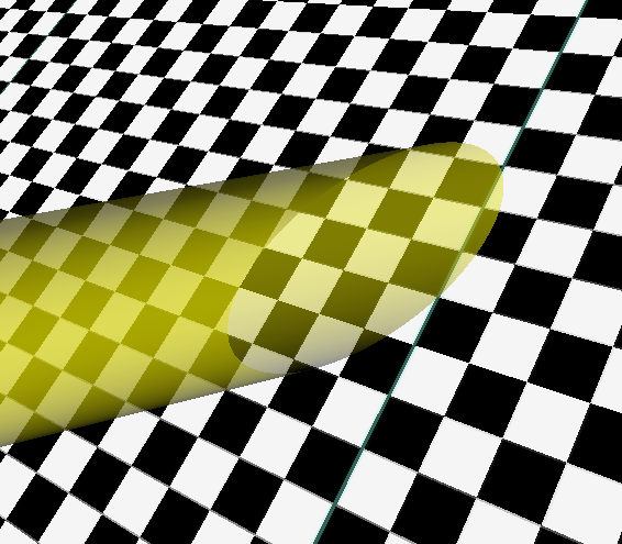
Texturing One Triangle
perspectively incorrect
perspectively correct
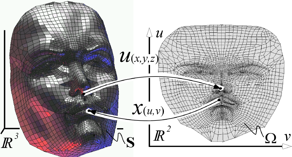
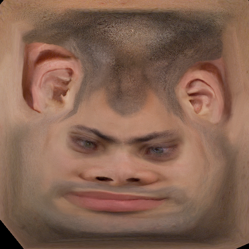
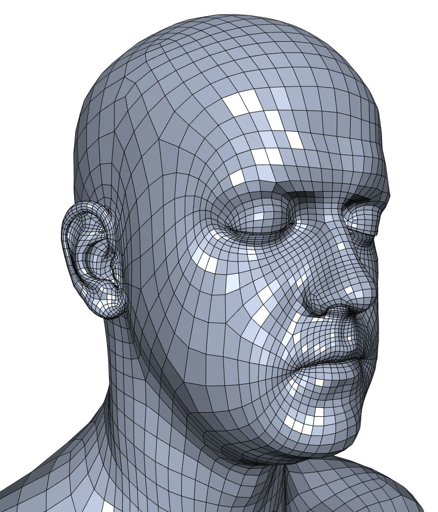
Texturing a Triangle Mesh
- How to find texture coordinates for each vertex?
- Find parameterization: Mapping between 2D texture space and 3D object space
- See lecture 3D Geometry Processing (Spring)
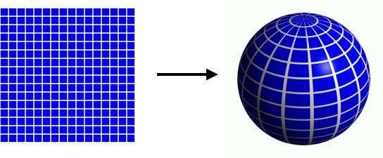
Simple Parameterizations
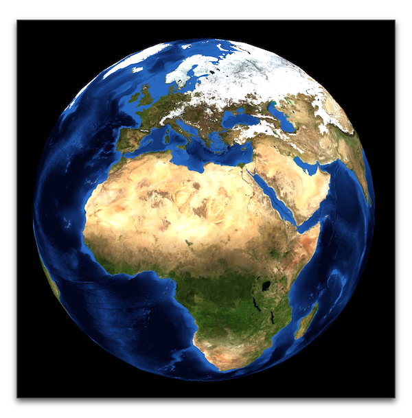
Sphere Parameterization
\[ \vector{ \phi \\ \theta } \mapsto \vector{ \cos\phi \, \cos\theta \\ \sin\phi \, \cos\theta \\ \sin\theta } \]
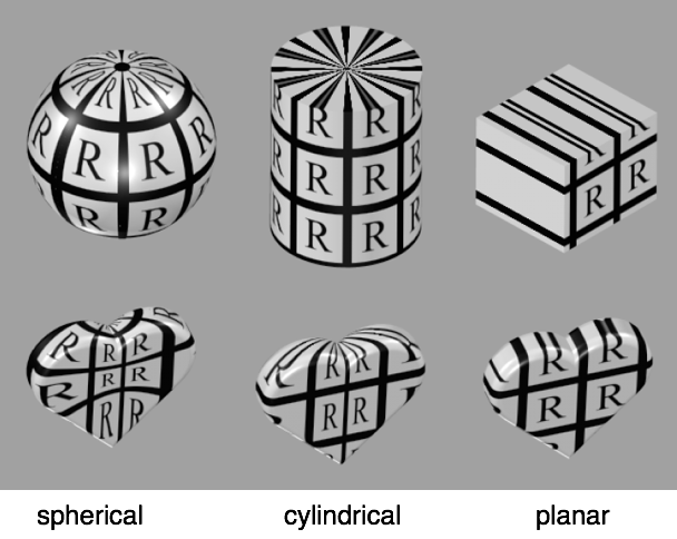
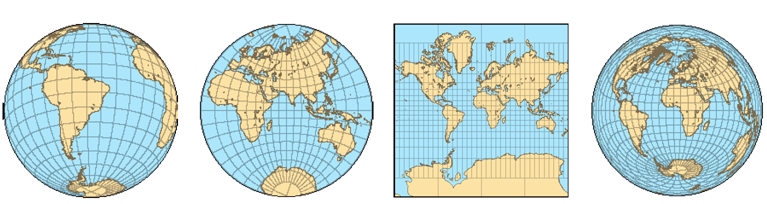
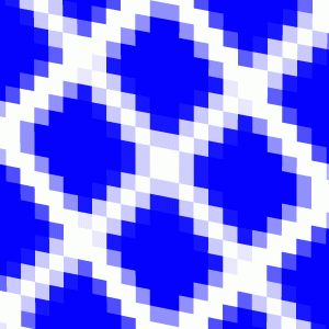
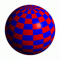
Cartography
- Many ways to parameterize a sphere!
- Some parameterizations have special properties:
- preserve angles (conformal, 2nd image)
- preserve areas (equi-areal, 4th image)
Low-Distortion Parameterization
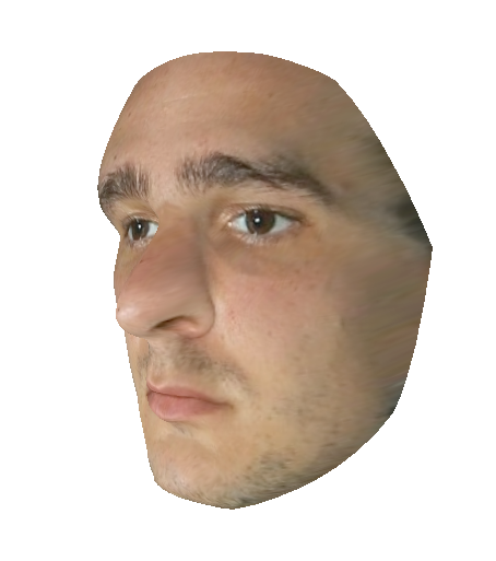

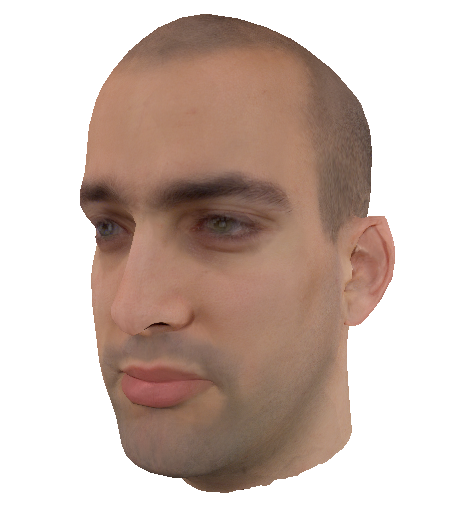
Low-Distortion Parameterization
Texture Interpolation
- How to get color value from real-valued texture coordinates \((u,v)\), such as \((u,v) = (6.4, 3.7)\)?
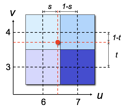
Round to nearest integer coordinate
color = tex[6,4];
Bilinear interpolation of neighboring texture pixels
color = (1-s)*(1-t)*tex[6,3] + (1-s)*t*tex[6,4]
              s*(1-t)*tex[7,3] +     s*t*tex[7,4];
Magnification Filter
 nearest
 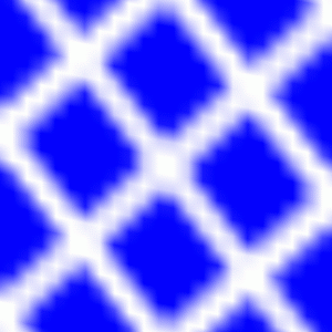 linear
Magnification Filter
 nearest
  linear
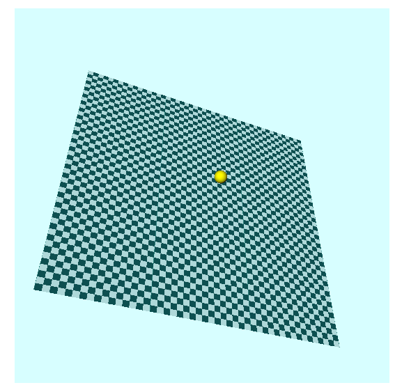
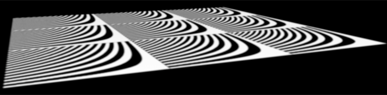
Minification Filter
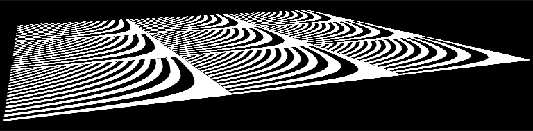
Minification Filter
- Point sampling is the wrong model
- Texture minification leads to aliasing
- Integrate over image pixel’s area in texture space
- Approximated by an ellipse
- Elliptically weighted averaging (EWA filtering)
Minification Filter
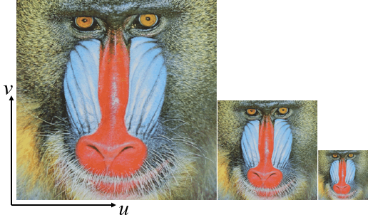
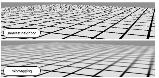
Mip-Mapping
- Store texture at multiple levels-of-detail
- MIP comes from the Latin “multum in parvo”: a multitude in a small space.
- Precompute down-scaled versions of texture image
- Use lower-resolution versions when far from camera
- OpenGL picks the most suitable image resolution for each per-pixel texture lookup based on pixel’s depth value
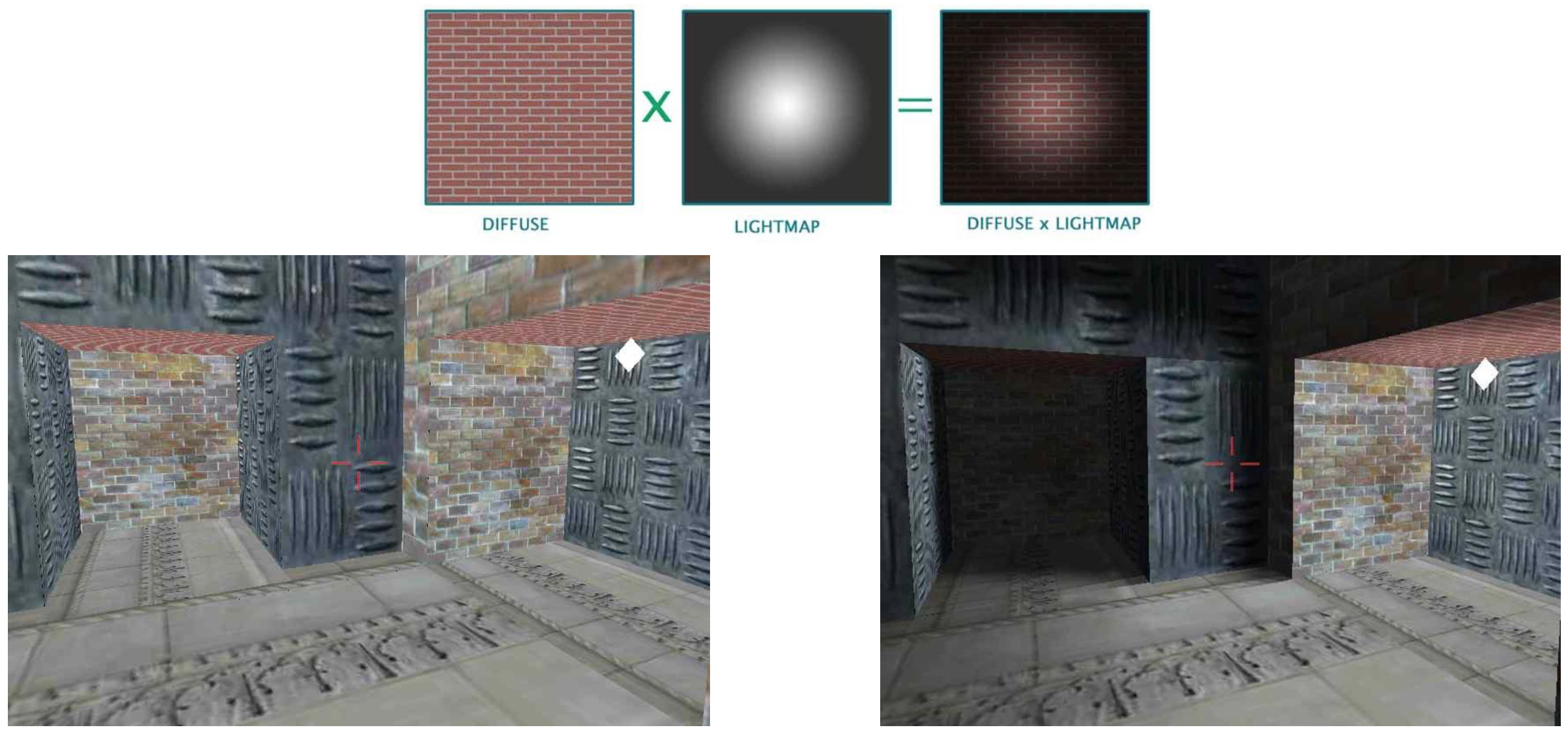
Light Maps
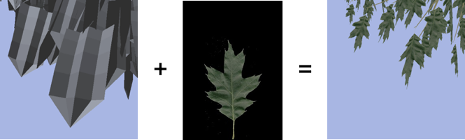
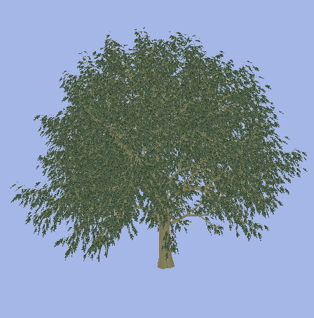
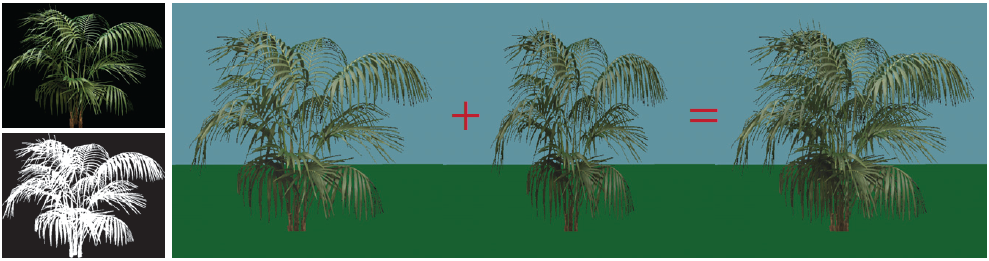
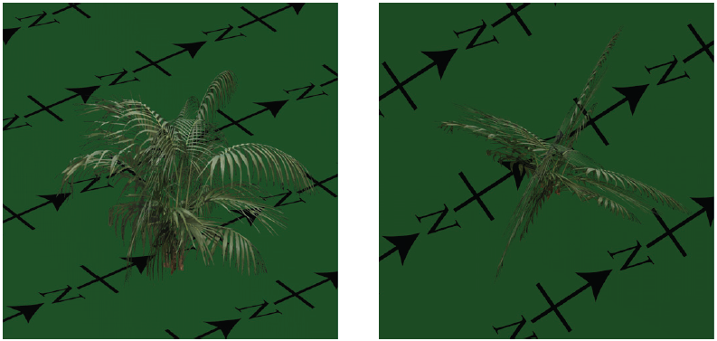
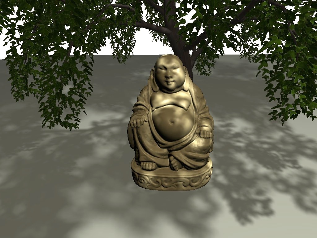
Alpha Maps
- Discard transparent texture pixels (alpha=0) in fragment shader. Frequently used for real-time rendering of plants.
Alpha Maps
- Discard transparent texture pixels (alpha=0) in fragment shader. Frequently used for real-time rendering of plants.
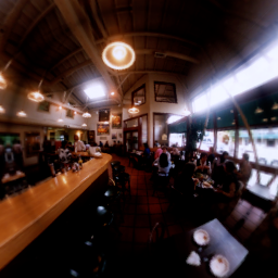
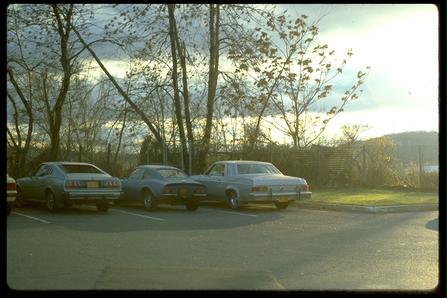
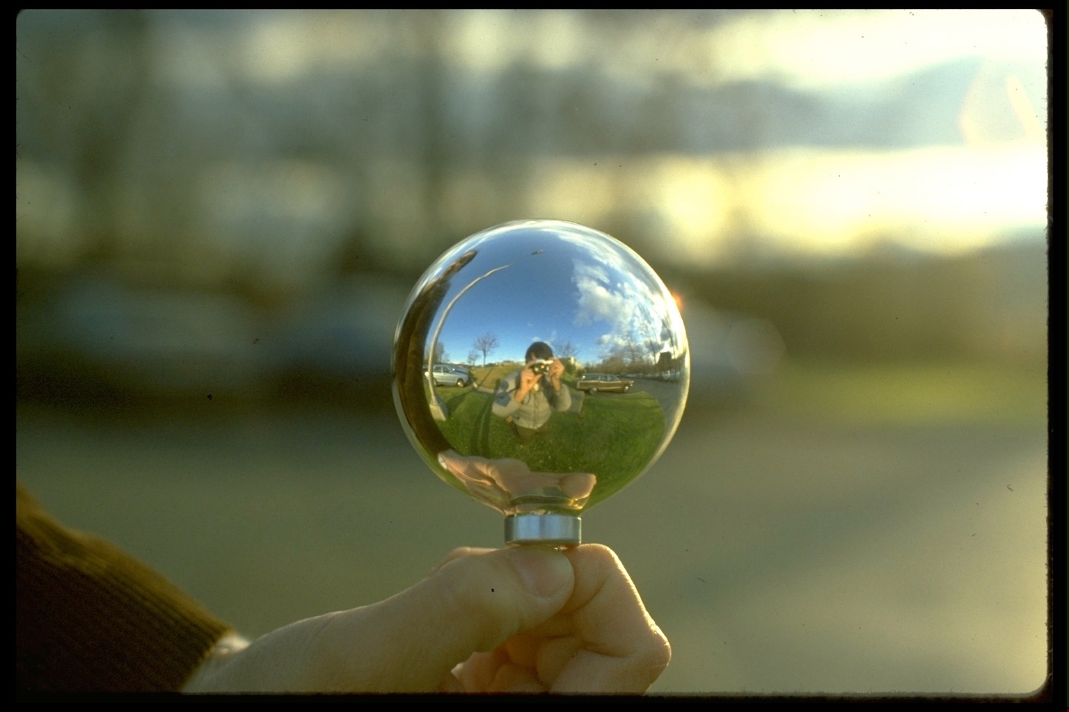
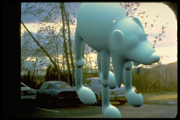
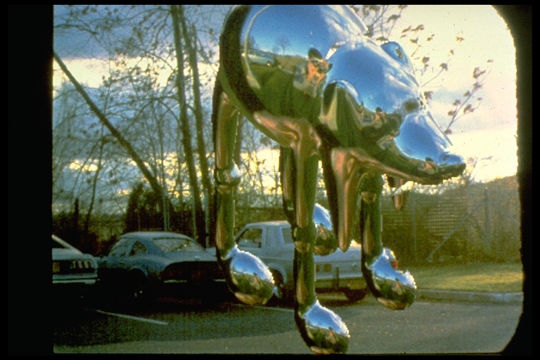
Environment Maps
- Approximate reflections of environment at surface.
- Environment is assumed to be far away from object.
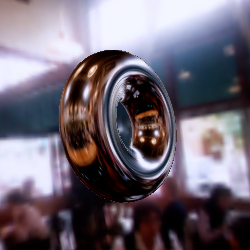
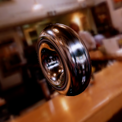
Spherical Environment Maps
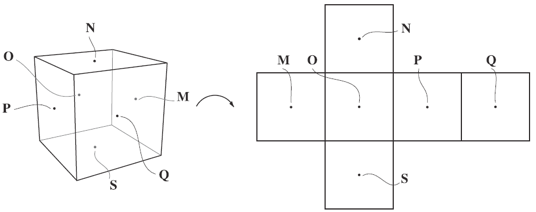
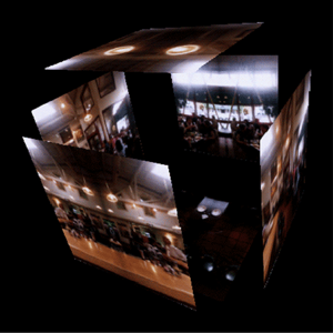
Cube Environment Maps
- Cube maps are the preferred representation.

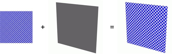
Bump Maps
- Add surface detail without increasing geometric complexity
- Perturb surface normal before lighting
- Assume bumps are small compared to geometry
- Bump pattern is taken from a texture
 normal rendering
 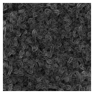 bump map
 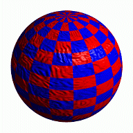 bump-mapped result
Bump Maps
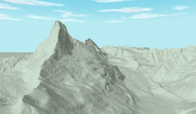
 Coarse mesh
 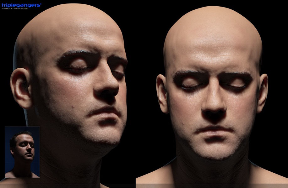 Diffuse map + specular map + bump map + …map
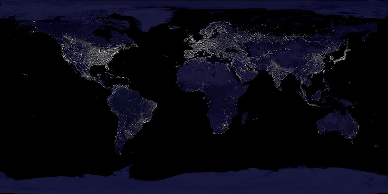
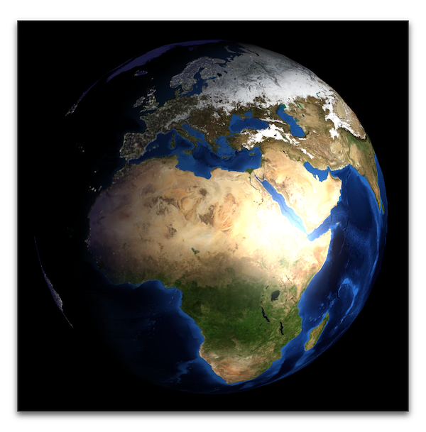
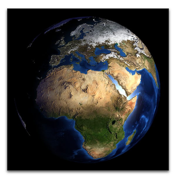
Nice Earth Textures
- NASA project Blue Marble: Next Generation
- Merged from many input images (from 2004)
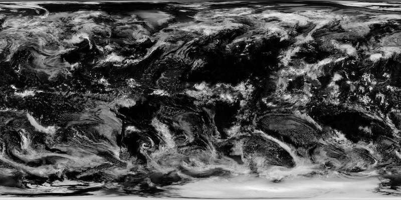
- Monthly day textures, night texture, clouds, …
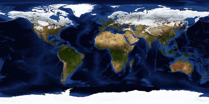
2D Texture
+ Diffuse and Specular Lighting
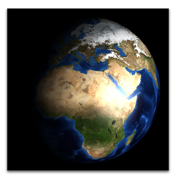
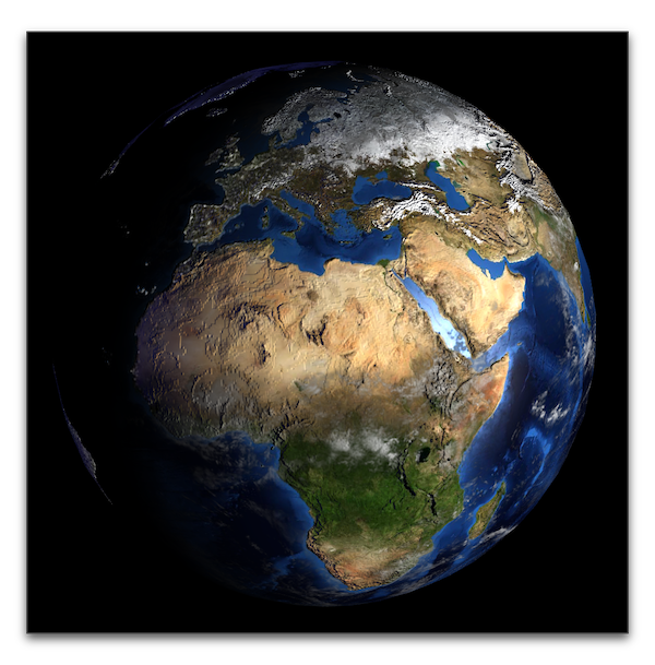
+ Night Texture
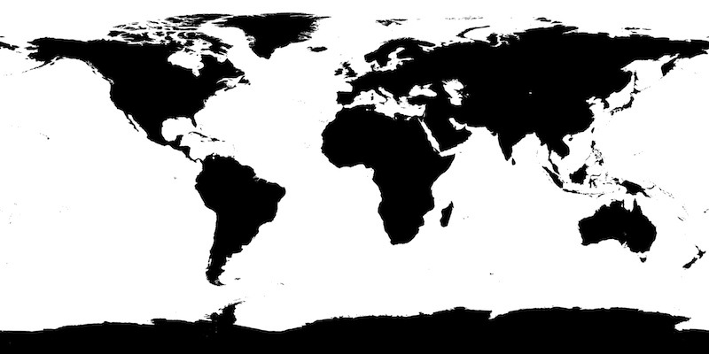
+ Specularity Map
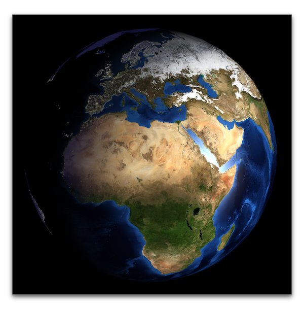
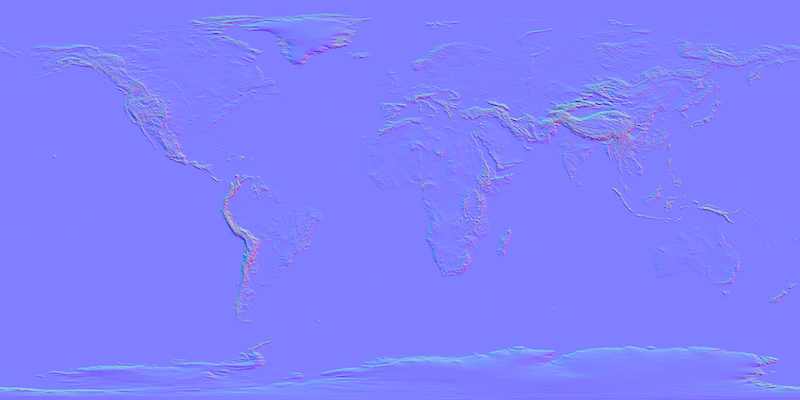
+ Normal Map
+ Clouds
Acknowledgments
Many thanks to Hartmut Schirmacher for providing aligned textures and initial WebGL code!

Beuth Hochschule für Technik Berlin
Literature
- Akenine-Möller, Haines, Hoffman: Real-Time Rendering, Taylor & Francis, 2008.
- Chapter 6
- Shreiner, Seller, Kessenich, Licea-Kane: OpenGL Programming Guide, 8th edition, 2013.
- Chapter 6

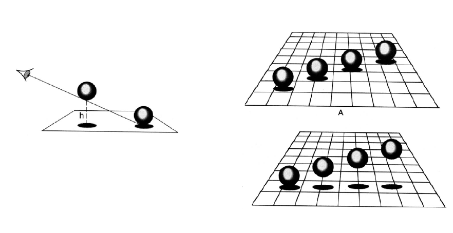
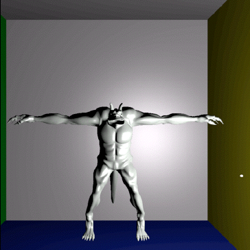
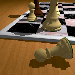
Shadows
- Shadows are important for 3D depth perception
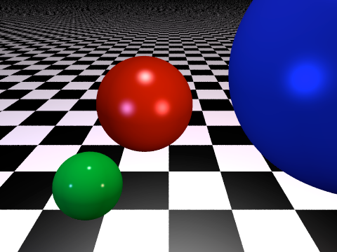
Shadows
- Shadows are important for 3D depth perception
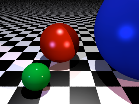
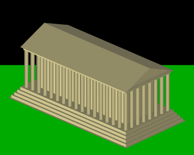
Shadows
- Shadows are important for 3D depth perception
Shadows
- Shadows are important for 3D depth perception
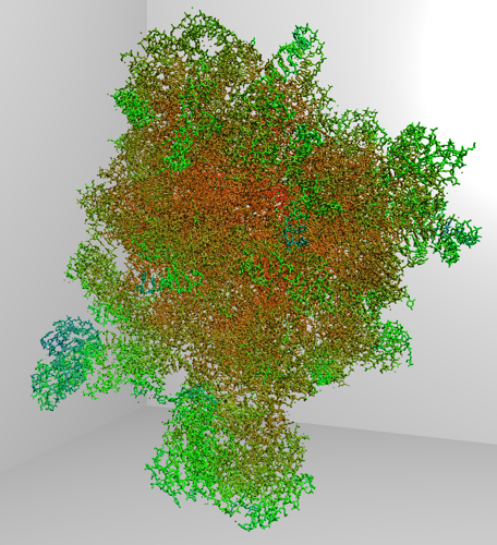
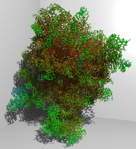
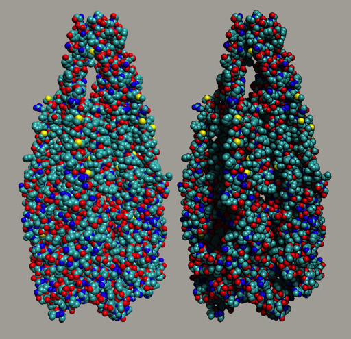
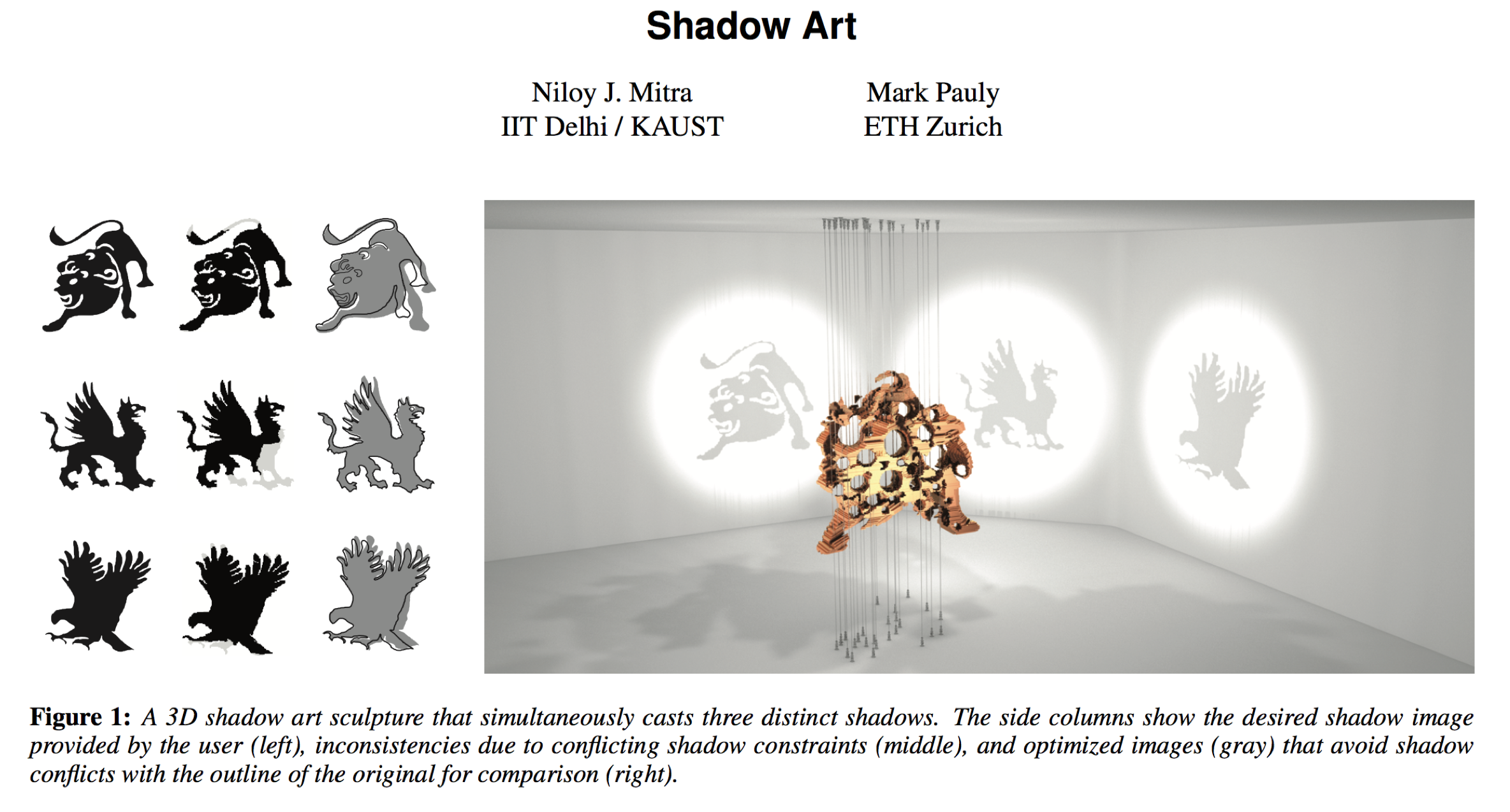
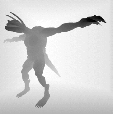
Shadow Art
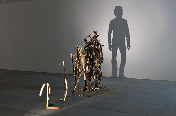
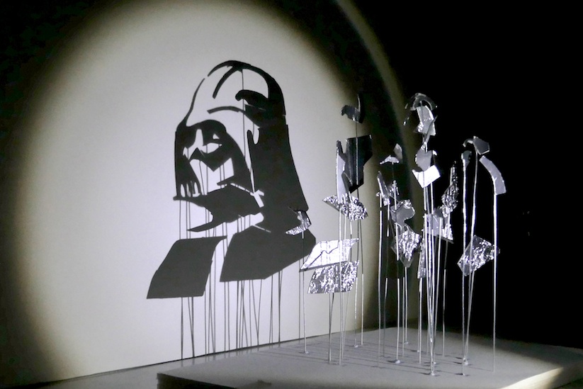
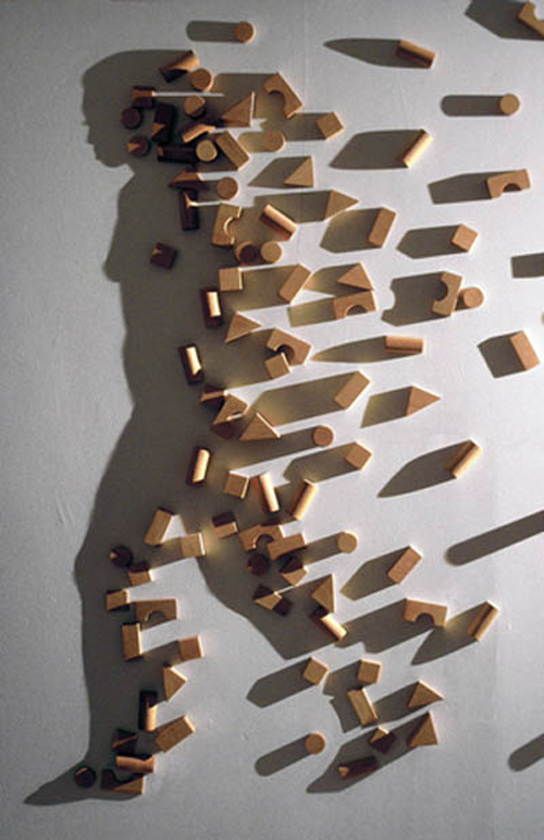
Shadow Art Research
Light Maps & Shadows
- Store precomputed lighting in textures
- Precomputation can take shadows into account
- Works for static scenes only
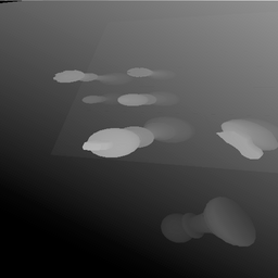
Shadow Maps
- Render scene as seen from light source
- Store z-buffer (holds distance to light)
- Light’s z-buffer is called shadow map
Shadow Maps
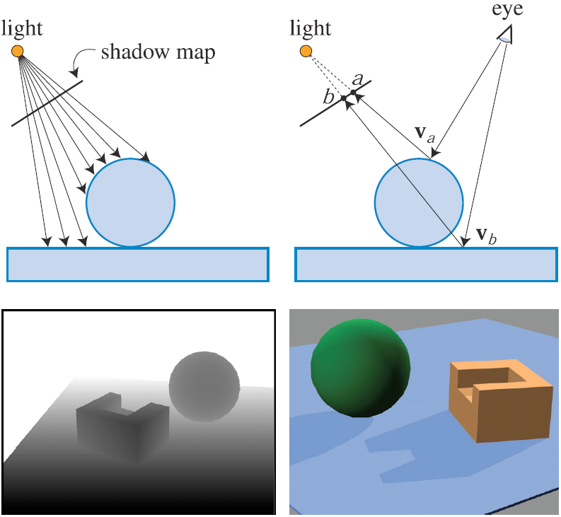
Shadow Maps
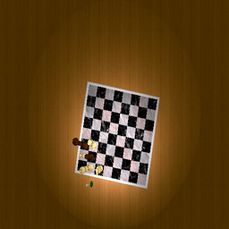
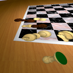
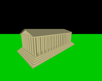 Scene without shadows
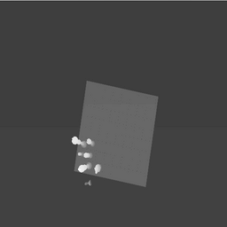
 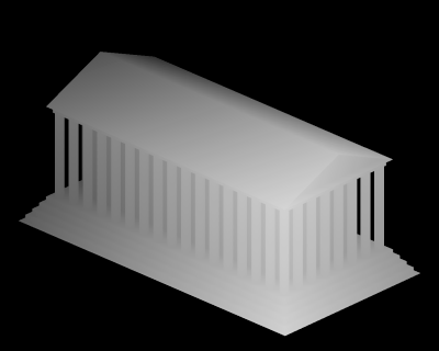 z-buffer of light’s view
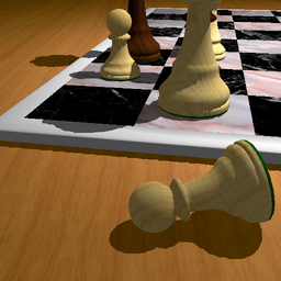
 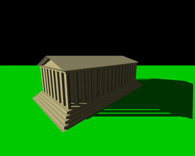 Scene with shadows
 Seen from light’s view
 ![]() Pixels in shadow
Pixels in shadow
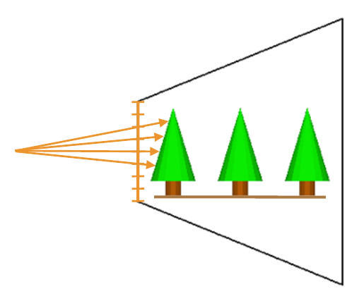
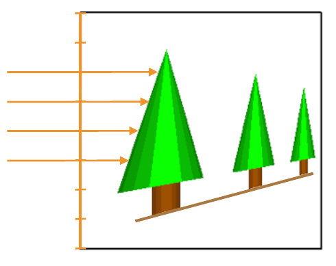
Shadow Map Aliasing
Perspective Shadow Maps
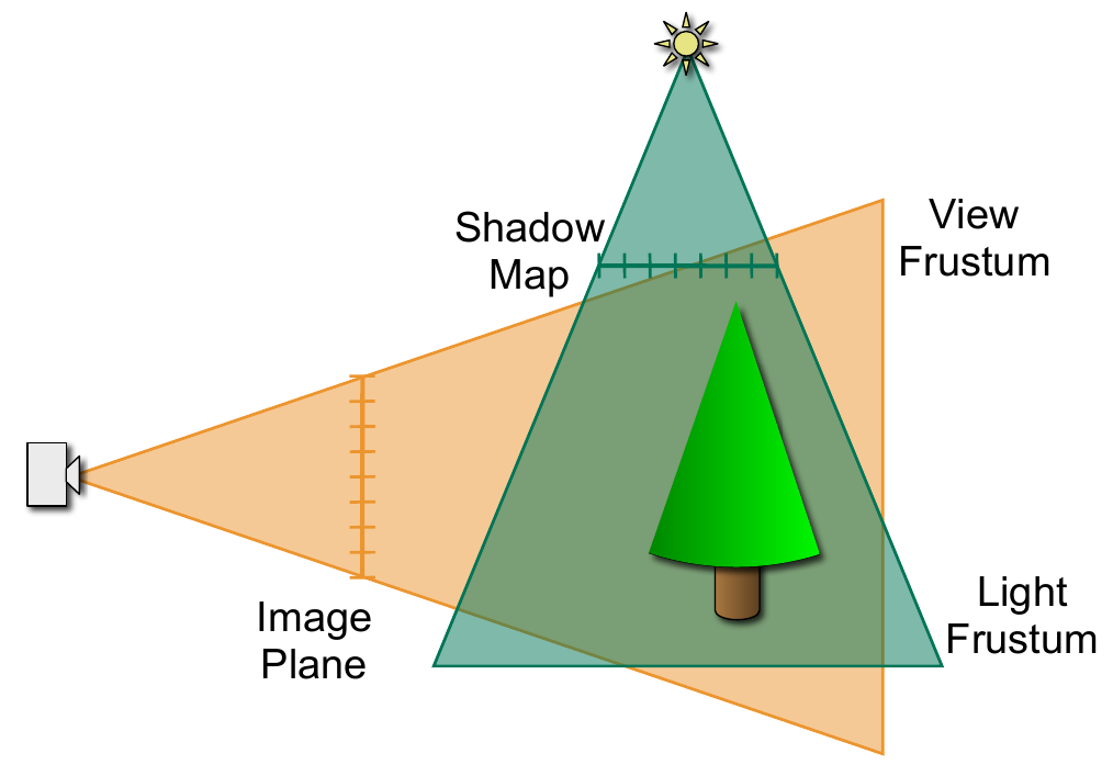
Projection Aliasing
Perspective Aliasing
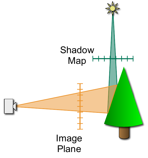
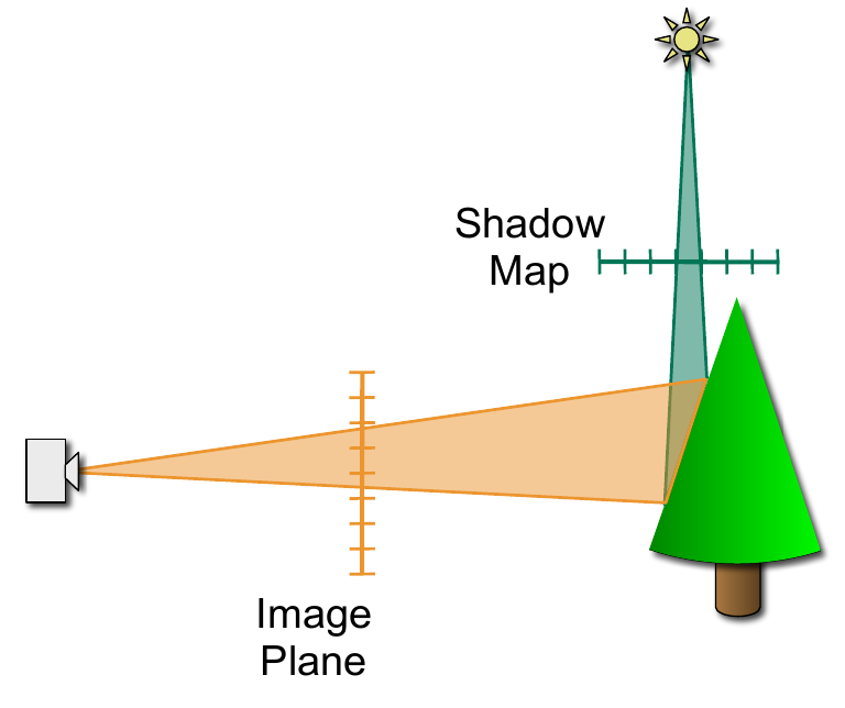
Perspective Shadow Maps
Perspective Shadow Maps
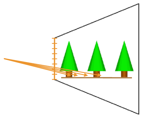
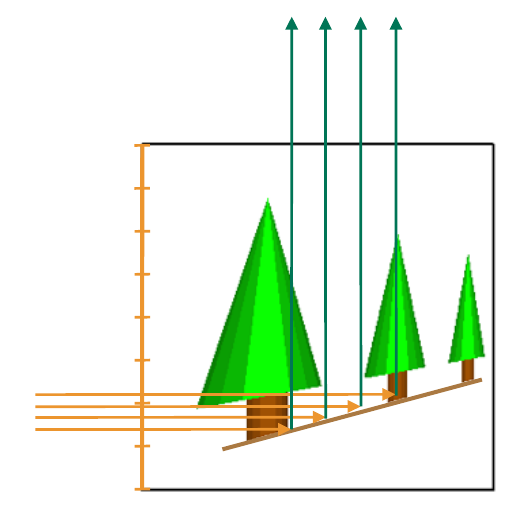
Perspective Shadow Maps
Soft Shadows?
Literature
- Hughes et al.: Computer Graphics: Principles and Practice, 3rd Edition, Addison-Wesley, 2014.
- Chapters 5.6, 15

- Shreiner et al: OpenGL Programming Guide, 8th edition, Addison-Wesley, 2013.
- Chapter 7
- Nvidia GPU Gems
- Chapter Perspective Shadow Maps: Care and Feeding