Computer Graphics

Rasterization in Detail

Prof. Dr. David Bommes

Computer Graphics Group

Last Time: 3D Transformations and Projections

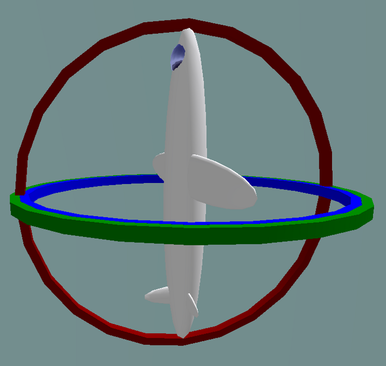
Rotation around x/y/z axes

Can we compose any 3D rotation from \(\mat{R}_x\), \(\mat{R}_y\), \(\mat{R}_z\)? \[ \mat{R}\of{\alpha, \beta, \gamma} \;\stackrel{?}{=}\; \mat{R}_x\of{\alpha} \cdot \mat{R}_y\of{\beta} \cdot \mat{R}_z\of{\gamma}\]

This representation is called Euler angles
- Often used in flight simulators: roll, pitch, yaw
- Problem: gimbal lock!

Wikipedia:Gimbal Lock

Rodrigues’ Rotation Formula

Rotation by angle \(\theta\) around (normalized) axis \(\vec{n}\)

\[ \mat{R}\of{\vec{n}, \theta} \;=\; \vec{n}\transpose{\vec{n}} + \cos\theta\left( \mat{I}-\vec{n}\transpose{\vec{n}} \right) + \sin\theta\,\underbrace{\matrix{ 0 & -n_z & n_y \\ n_z & 0 & -n_x \\ -n_y & n_x & 0 }}_{=\mat{N}} \]

Combining the three matrices and writing \(\vec{n}=(x,y,z), c=\cos\theta, s=\sin\theta\) gives

\[ \mat{R}\of{\vec{n}, \theta} \;=\; \matrix{ x^2(1-c)+c & xy(1-c)-zs & xz(1-c)+ys \\ yx(1-c)+zs & y^2(1-c)+c & yz(1-c)-xs \\ xz(1-c)-ys & yz(1-c)+xs & z^2(1-c)+c } \]

Wikipedia

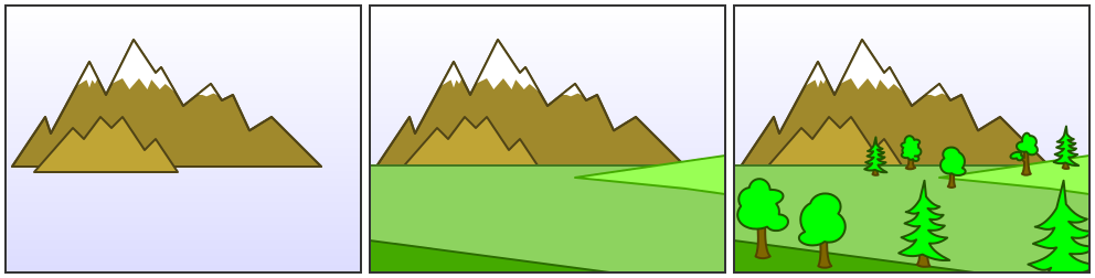
Transformation Pipeline

View Transformation
- setup extrinsic camera parameters: position and orientation
Projection Transformation
- setup intrinsic camera parameters: opening angle and depth range
Viewport Transformation
- setup image parameters/resolution: width and height

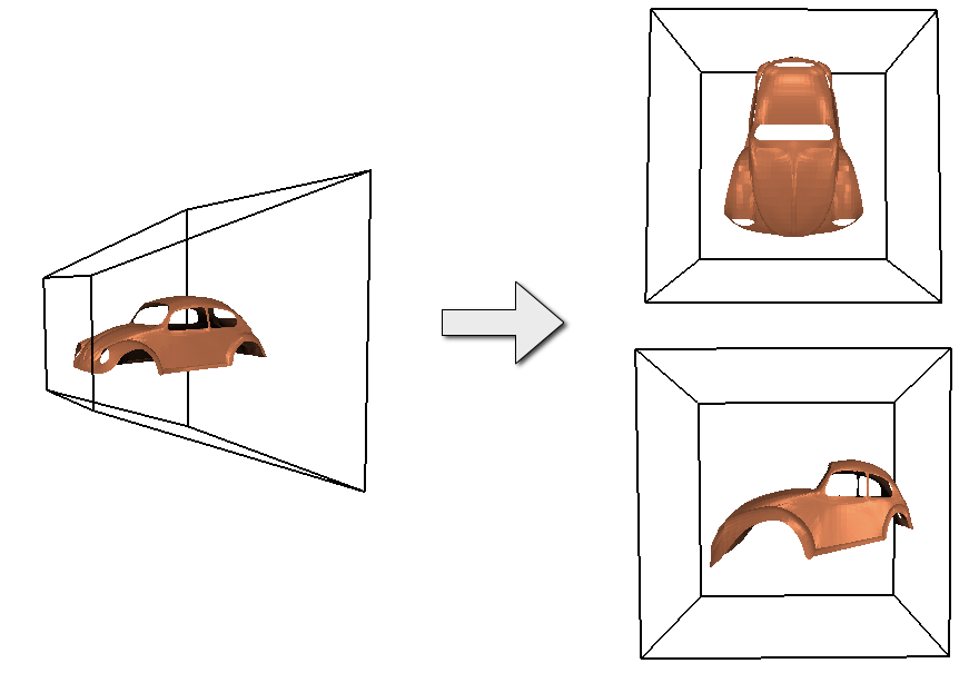
Generic Perspective Projection

Standard projection
- Center of projection: \((0,0,0)\)
- Image plane at \(z=-d\)

\[ \vector{x\\y\\z} \;\mapsto\; \vector{x \cdot \frac{-d}{z} \\ y \cdot \frac{-d}{z} \\ -d} \quad\longleftrightarrow\quad \matrix{ 1 & 0 & 0 & 0 \\ 0 & 1 & 0 & 0 \\ 0 & 0 & 1 & 0 \\ 0 & 0 & -1/d & 0 } \cdot \vector{x\\y\\z\\1} \;=\; \vector{x\\y\\z\\-z/d} \;\cong\; \vector{x \frac{-d}{z} \\ y \frac{-d}{z} \\ -d\\ 1} \]

Homogeneous Coordinates

Use homogeneous coordinates \((x,y,z,w)\)!
- Vectors are represented by \(\transpose{(x,y,z,0)}\)
- Points are represented by \(\transpose{(wx,wy,wz,w)}\) for any \(w \neq 0\)
Divide a point \(\transpose{(wx,wy,wz,w)}\) by \(w\) to get its canonical representation \(\transpose{(x,y,z,1)}\) (“homogenization”)
- Defer homogenization until the very last step
We can now use \(4 \times 4\) matrices for
- linear transformations (scaling, rotation)
- affine transformations (linear map + translation)
- projective transformations (affine map + projection)

Today: Rasterization Details

Rasterization Pipeline

Ray Tracing vs. Rasterization

Ray Tracing
- Shoot rays from 2D pixels into 3D scene
- “backward rendering”
- needs ray intersections

Rasterization
- Project 3D objects onto 2D image plane
- “forward rendering”
- needs transformations & projections

images/raytracing-vs-rasterization-2.svg

Rasterization Pipeline

Transformations & Projections

Transformations & Projections

Project line or triangle from 3D to 2D
- Simply transform/project its endpoints/vertices
- Why is this correct?

Let us first analyze this for a line between \(\vec{A}\) and \(\vec{B}\) \[ \vec{X}\of{\alpha} = (1-\alpha) \vec{A} + \alpha \vec{B} \]

For an affine/projective transformation \(\mat{M}\) it has to hold \[ \forall \alpha \in \R \;\; \exists \beta \in \R \;:\; \mat{M}\of{\vec{X}\of{\alpha}} \;=\; (1-\beta)\mat{M}\of{\vec{A}} + \beta \mat{M}\of{\vec{B}} \]

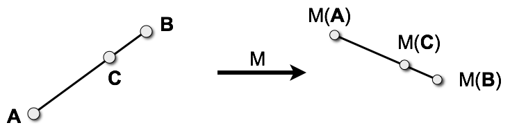
Affine Transformations of Lines

Affine transformation \(\mat{M}\) preserves affine combinations \[ \mat{M}\of{(1-\alpha)\vec{A} + \alpha\vec{B}} \;=\; (1-\alpha)\mat{M}\of{\vec{A}} + \alpha\mat{M}\of{\vec{B}} \]

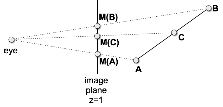
Projective Transformations of Lines

For a central projection \(\mat{P}(\vec{X}) = \frac{\vec{X}}{\vec{X}_z}\) we can show that
\(\mat{P}\of{\vec{X}\of{\alpha}} = \frac{(1-\alpha)\vec{A} + \alpha\vec{B}}{(1-\alpha)\vec{A}_z + \alpha\vec{B}_z} = (1-\beta) \frac{\vec{A}}{\vec{A}_z} + \beta \frac{\vec{B}}{\vec{B}_z}\)
if we chose \(\beta \;=\; \frac{\alpha\vec{B}_z}{(1-\alpha)\vec{A}_z + \alpha\vec{B}_z}\)
Same argument holds for general projective transformations.

Transformations of Triangles

A triangle is an affine combination of three points \[ \vec{X}\of{\alpha, \beta, \gamma} \;=\; \alpha\vec{A} + \beta\vec{B} + \gamma\vec{C}\]
with \(\alpha+\beta+\gamma=1\).
Affine transformation preserve affine combinations
- Triangles are transformed to triangles
Planar projections map triangles to triangles
- Similar derivation as for lines

Lighting

Normal Vectors

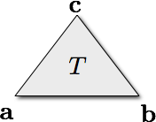
Triangle normal \[ \vec{n}(T) = \frac{\left(\vec{b}-\vec{a}\right) \times \left(\vec{c}-\vec{a}\right)} {\norm{\left(\vec{b}-\vec{a}\right) \times\left(\vec{c}-\vec{a}\right)}} \]

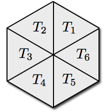
Vertex normal \[ \vec{n}(V) = \frac{ \sum_{T_i \ni V} w(T_i) \, \vec{n}(T_i)} { \norm{ \sum_{T_i \ni V} w(T_i) \, \vec{n}(T_i)} } \]

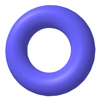
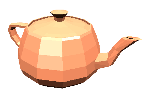
Vertex Normals

triangulation (flat shading) images/vertex-normals-2.png

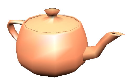
no weighting images/vertex-normals-3.png

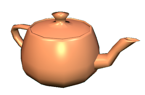
angle-weighted

Phong Lighting Model

Ambient lighting
- approximate global light transport / exchange
- uniform in, uniform out

Diffuse lighting
- dull / matt surfaces
- directed in, uniform out

Specular lighting
- shiny surfaces
- directed in, directed out

Phong Lighting Model

images/torus-a.png ambient: \(I_a m_a\) 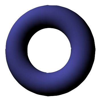images/torus-d.png diffuse: \(I_l m_d \left( \vec{n} \cdot \vec{l} \right)\) 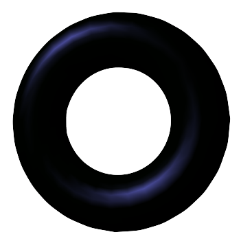images/torus-s.png specular: \(I_l m_s \left( \vec{r} \cdot \vec{v} \right)^s\)

\[ I \;=\; I_a m_a + I_l \left( m_d \left( \vec{n} \cdot \vec{l} \right) + m_s \left( \vec{r} \cdot \vec{v} \right)^s \right) \]

How to transform normal vectors?

A point \(\vec{x} = \transpose{(x,y,z,1)}\) lies on its tangent plane, specified by \(\vec{n} = \transpose{(n_x, n_y, n_z, d)}\): \[ n_x x + n_y y + n_z z + d = 0 \quad\Leftrightarrow\quad \transpose{\vec{n}} \vec{x} = 0 \]

The same equation should be satisfied after an affine transformation \(\mat{M}\) maps \(\vec{x}\) to \(\vec{x}'\) and \(\vec{n}\) to \(\vec{n}'\) \[ 0 \;=\; \transpose{\vec{n}'} \vec{x}' \;=\; \transpose{\vec{n}'} \mat{M} \vec{x} \;=\; \transpose{\left(\transpose{\mat{M}} \vec{n}' \right)} \vec{x} \]

Comparing the two equations yields \(\vec{n}' = \mat{M}^{\mathsf{-T}} \vec{n}\)
- In practice use upper-left \(3 \times 3\) block of \(\mat{M}\)
- Don’t forgot to re-normalize \(\vec{n}'\)

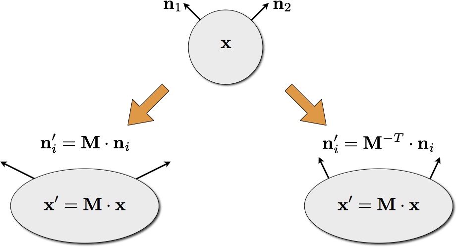
How to transform normal vectors?

Clipping

Rasterization

Line Rasterization

Discretize line from \((x_0, y_0)\) to \((x_1, y_1)\) to pixel grid.
- Endpoints are integer coordinates (pixel positions)
- Assume slope is in \([0,1]\) and \(x_0 < x_1\)
- Other cases follow by symmetry

How would you implement this?

Line Representation

Explicit representation
- Range of a function \(y(x) = m\,x + t\)
  
  with \(m = \frac{y_1-y_0}{x_1-x_0}\) and \(t = y_0 - m\,x_0\)

First Guess

for (x=x0; x<=x1; ++x)
	set_pixel(x, round(m*x + t));

Bad: Multiplication & Rounding

Digital Differential Analysis

Use an incremental algorithm!
If the current pixel is \((x_i, y_i)\) then
- \(x_{i+1} = x_i + 1\)
- \(y_{i+1} = y_i + m\)

for (x=x0, y=y0; x<=x1; ++x, y+=m)
	set_pixel(x, round(y));

Good: no multiplication
Bad: rounding, since \(y\) and \(m\) are floats

Line Representations

Explicit representation
- Range of a fuction \(y(x) = m\,x + t\)
  with \(m = \frac{y_1-y_0}{x_1-x_0}\) and \(t = y_0 - m\,x_0\)

Implicit representation
- Zero-set of a function \(F(x,y) = ax + by + c\)
  with \(a = (y_1-y_0)\), \(b = (x_0-x_1)\), \(c = t \, (x_1-x_0)\)
- \(F(x,y) = 0\) \(\Longrightarrow\) point on line
- \(F(x,y) > 0\) \(\Longrightarrow\) point below line
- \(F(x,y) < 0\) \(\Longrightarrow\) point above line

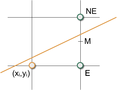
Bresenham Algorithm

Next pixel can only be east (E) or north-east (NE)
- Is the line below/above midpoint \(\vec{M}\)?

Use a decision variable \(d\):
- \(d = F(M) = F(x_i+1, y_i+0.5)\)
- If \(d \leq 0\) then go east
- If \(d > 0\) then go north-east

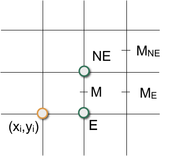
Bresenham Algorithm

Incrementally update decision variable \(d\)!

If east was chosen:
- \(d_\mathrm{new} = F(x_i+2, y_i+0.5) = d_\mathrm{old} + a\)
- \(\Delta\mathrm{E} := a = \Delta y\)
If north-east was chosen:
- \(d_\mathrm{new} = F(x_i+2, y_i+1.5) = d_\mathrm{old} + a + b\)
- \(\Delta\mathrm{NE} := a + b = \Delta y - \Delta x\)

Bresenham Algorithm

Initialization of \(d\)
- \(d = F(x_0+1, y_0+0.5) = \Delta y - \Delta x / 2\)
- Bad: \(\Delta x / 2\) may not be integer

Use \(2 \cdot F(x,y)\) instead of \(F(x,y)\)
- Values of \(d\), \(\Delta\mathrm{E}\), \(\Delta\mathrm{NE}\) are doubled
- But sign of \(F\) and \(d\) remain unchanged

Bresenham Algorithm

Δx  = x1-x0;
Δy  = y1-y0;
d   = 2*Δy - Δx;
ΔE  = 2*Δy;
ΔNE = 2*(Δy - Δx);

set_pixel(x0, y0);

for (x = x0, y = y0; x < x1;)
{
	if (d <= 0)    { d += ΔE;  ++x;     }
	else           { d += ΔNE; ++x; ++y }
	set_pixel(x, y);
}

Good: Only integer arithmetic!

Why only integer arithmetic?

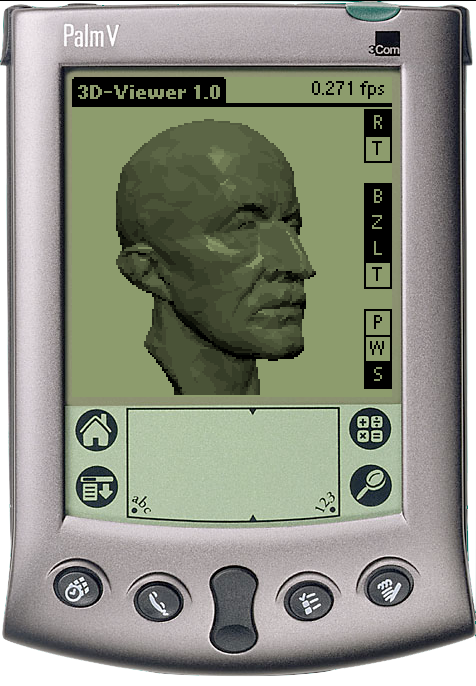
Crucial for systems without FPU

Triangle Rasterization

Enumerate all pixels inside a 2D triangle
- Inside test for every pixel is too expensive
Compute horizontal spans in each scanline
- Compute intersections with triangle edge, fill inbetween

Many special cases to consider!

Triangle Rasterization

Shading

Shading: Fill the Interior

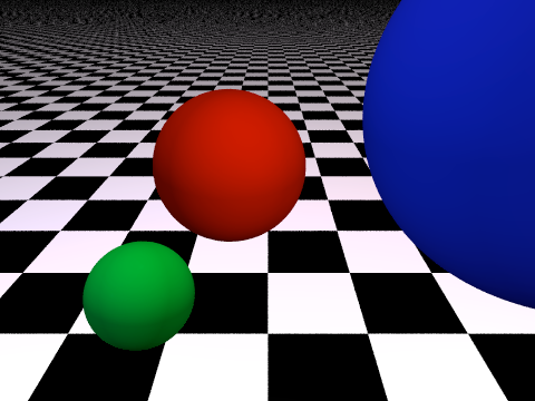
Flat Shading
- Compute Phong lighting per face
- Facetted appearance
- Mach band effect
Gouraud Shading
- Compute Phong lighting per vertex
- Linear interpolation of colors
- Looses small highlights
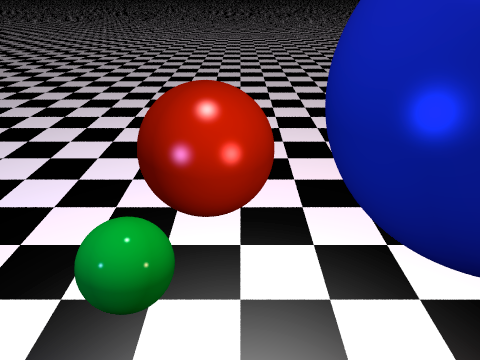
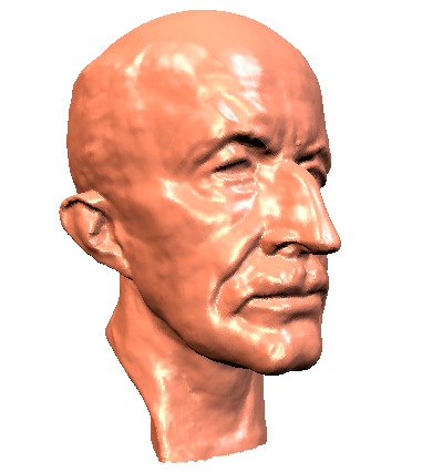
Phong Shading
- Linear interpolation of vertex normals
- Compute Phong lighting per pixel
- Captures small highlights

images/teapot-flat.png
images/teapot-gouraud.png
images/teapot-phong.png

Shading: Fill the Interior

Flat Shading images/cat-gouraud.png

Gouraud Shading images/cat-phong.png

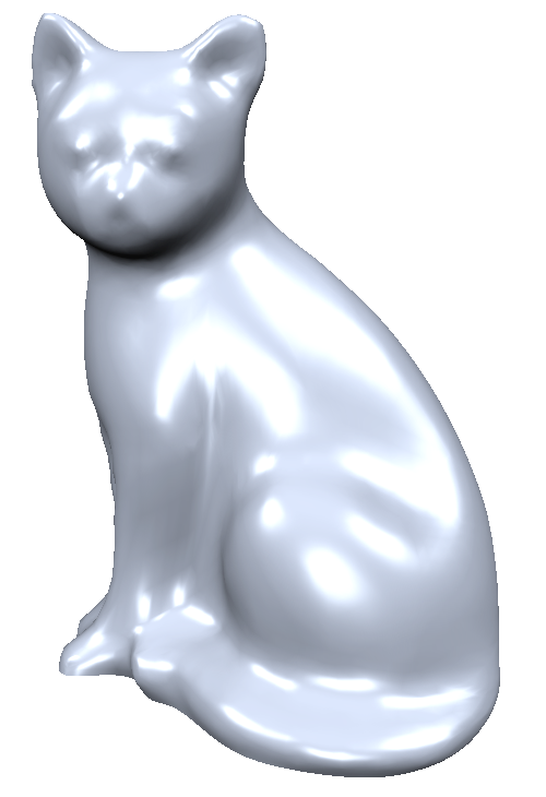Phong Shading

Shading: Fill the Interior

Visibility

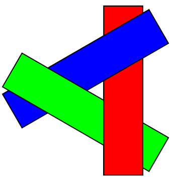
Painter’s Algorithm

Idea: How do painters paint?
- Draw objects/triangles from back to front
- Overwrites polygons in the back

Wikipedia

Painter’s Algorithm

Idea: How do painters paint?
- Draw objects/triangles from back to front
- Overwrites polygons in the back

Algorithm
- Sort all polygons w.r.t. \(z_\text{max}\) (farthest vertex)
- Disambiguate if \(z\)-ranges of polygons overlap
- Paint polygons from back to front
- Complexity: \(O(n \log n)\) for \(n\) polygons

Painter’s Algorithm

Disambiguate if \(z_\text{max}(A) > z_\text{max}(B) > z_\text{min}(A)\)
- Paint \(A\) if
  - \([x,y]\)-ranges not overlapping, or
  - Non-overlapping projections
  - \(A\) behind supporting plane of \(B\), or
  - \(B\) in front supporting plane of \(A\), or
- Swap \(A\) & \(B\)
  - \(B\) behind supporting plane of \(A\), or
  - \(A\) in front supporting plane of \(B\)

Painter’s Algorithm

Repeated swap → cyclic overlap
- Split \(A\) at supporting plane of \(B\) or vice versa

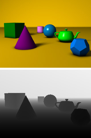
Z-Buffer

Store current min. z-value for each pixel
- After model transformation, view transformation, projection transformation, and viewport transformation
Additional buffer for depth values
- Framebuffer stores RBG color values
- Depth buffer (z-buffer) stores depth values
- Storage: additional 16 to 32 bits per pixel

Z-Buffer

Initialize depth buffer to \(\infty\)
Rasterize triangles, interpolate depth value per fragment
- each fragment (x,y) still has a depth value z
Depth buffer test & update

    // draw color rgb to pixel (x,y)
    void set_pixel(x, y, z, rgb)
    {
        // is current pixel closer than stored z-value?
        if (z < zbuffer[x,y])
        {
            // write pixel's color to frame buffer
            framebuffer[x,y] = rgb;

            // update depth buffer
            zbuffer[x,y] = z;
        }
    }

Z-Buffer

Complexity
- \(O(n)\) for \(n\) polygons
- How can we sort n polygons in linear time?
Most important visibility algorithm
- Implemented in hardware for all GPUs
- Used by OpenGL

Quiz: z-Buffer

How will the z-buffer resolve visibility when two triangles \(A\) and \(B\) lie in the same plane and overlap? Assume triangle \(A\) is drawn before triangle \(B\).

\(A\) will be completely visible.
\(B\) will be completely visible.
Some pixels from \(A\) and some pixels from \(B\) will be visible in the overlap region.
One triangle is completely visible, but it is random which one.

Z-Buffer

Z-fighting

Wikipedia

Quiz: z-Buffer

How does quantization of the z-values affect visibility inside the view volume?

z-testing has the same effective resolution in the entire view volume.
z-testing has more effective resolution close to the near plane.
z-testing has more effective resolution far from the near plane.

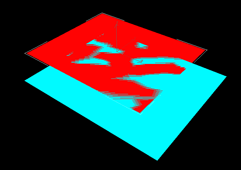
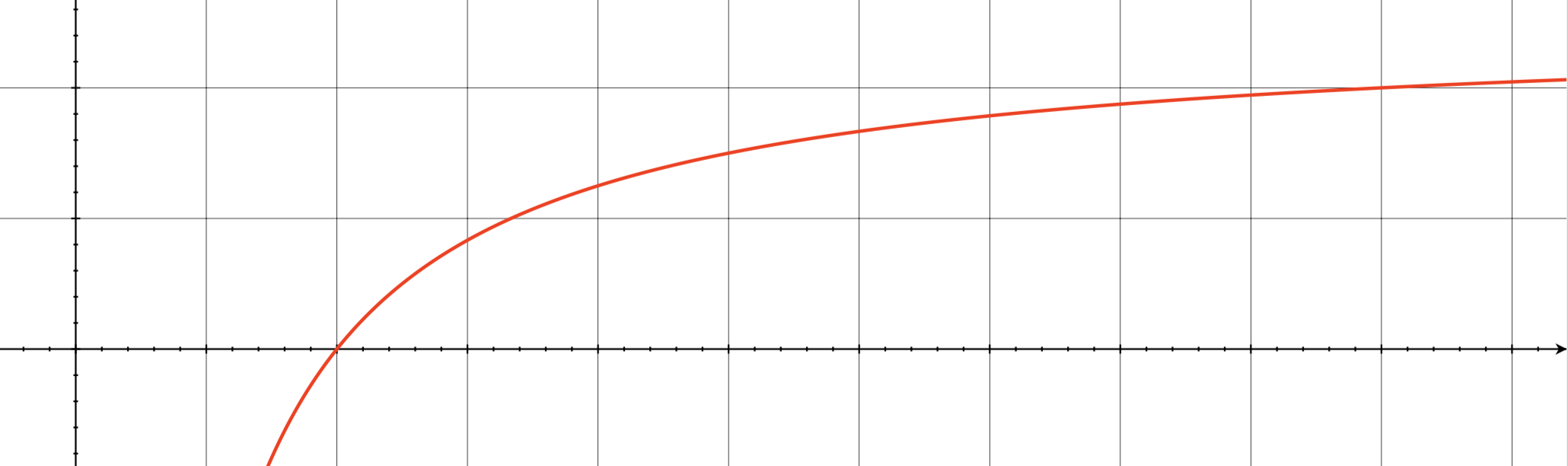
Z-Buffer

Higher resolution at near plane!

Depth Buffer Precision

Rasterization Pipeline

Ray Tracing vs. Rasterization

“Rasterization is fast, but needs cleverness to support complex visual effects. Ray tracing supports complex visual effects, but needs cleverness to be fast.”

– David Luebke, Nvidia

Literature

Hughes et al.: Computer Graphics: Principles and Practice, 3rd Edition, Addison-Wesley, 2014.
- Chapter 15