Computer Graphics
Triangle Meshes


Last Time: Lighting


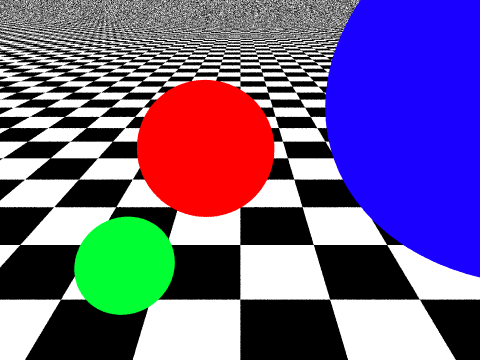 no illumination
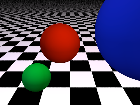
 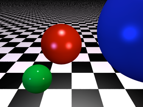 local illumination
 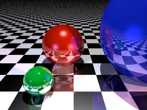 global illumination
Phong Lighting Model
- Ambient lighting
- approximate global light transport / exchange
- uniform in, uniform out
- Diffuse lighting
- dull / matt surfaces
- directed in, uniform out
- Specular lighting
- shiny surfaces
- directed in, directed out
Phong Lighting Model
 ambient: \(I_a m_a\)
 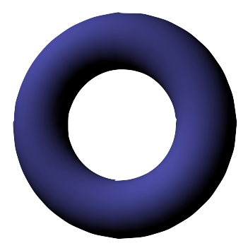 diffuse: \(I_l m_d \left( \vec{n} \cdot \vec{l} \right)\)
 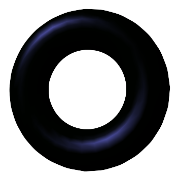 specular: \(I_l m_s \left( \vec{r} \cdot \vec{v} \right)^s\)

\[ I \;=\; I_a m_a + I_l \left( m_d \left( \vec{n} \cdot \vec{l} \right) + m_s \left( \vec{r} \cdot \vec{v} \right)^s \right) \]
Real or Rendered?

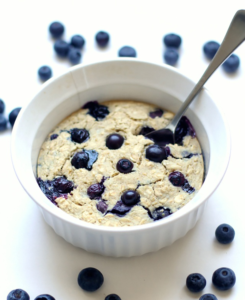
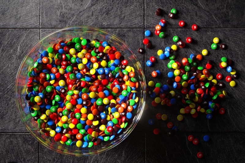


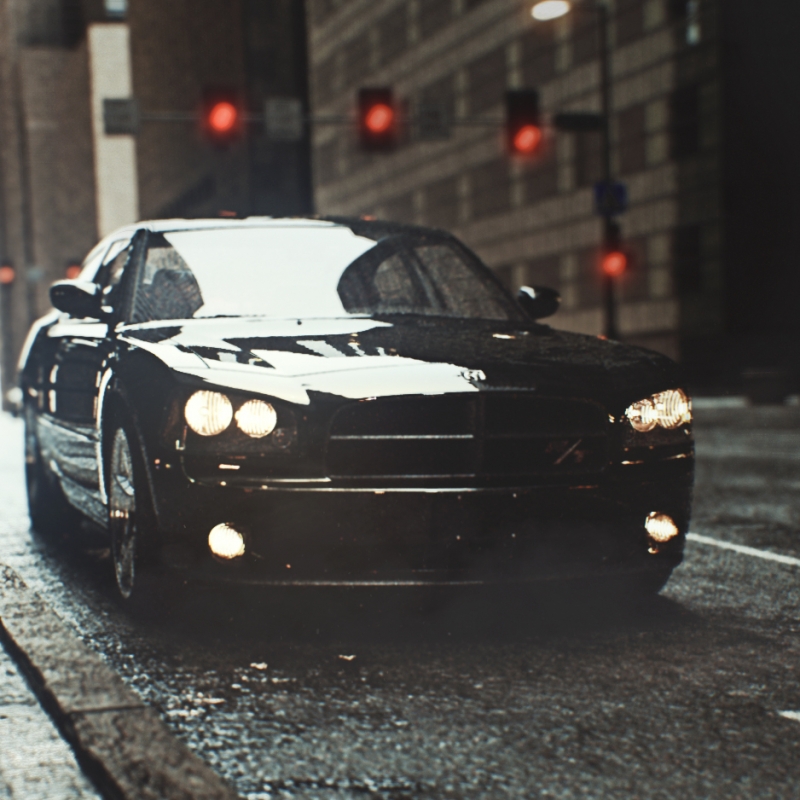
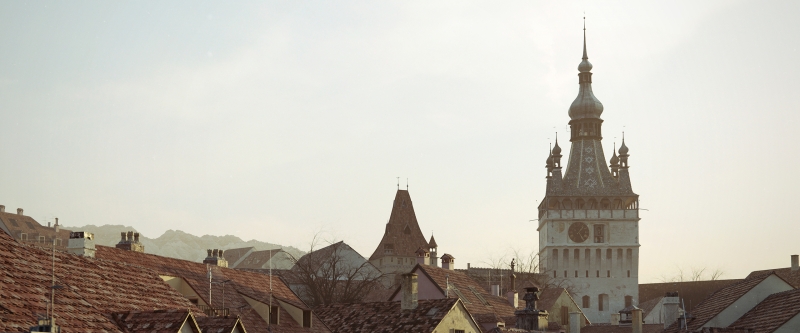
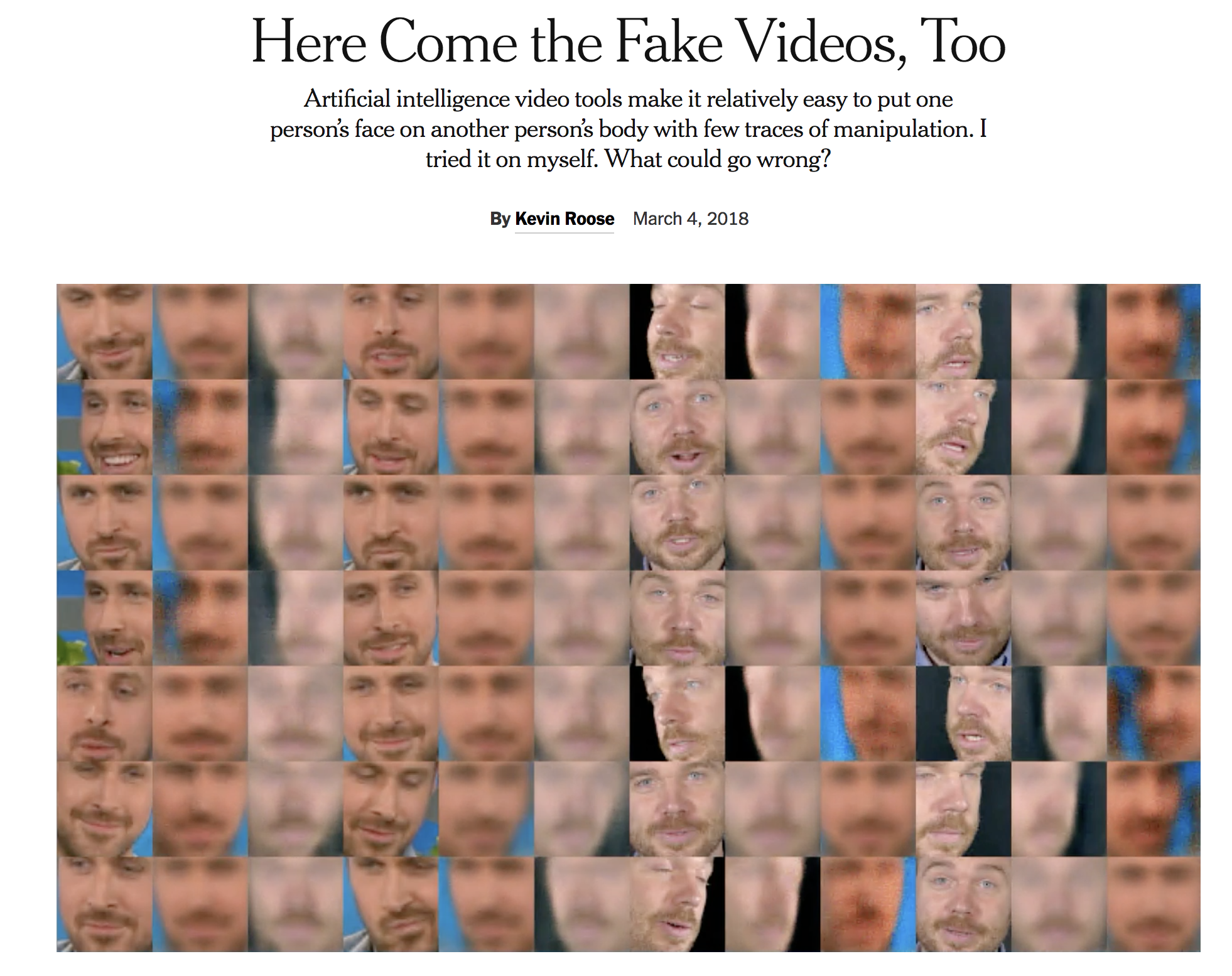
Fake Images and Videos
Today: Ray Tracing Meshes
- Extend ray tracing to triangle meshes
- Mesh data structures
- Lighting computations
- Efficient ray intersections

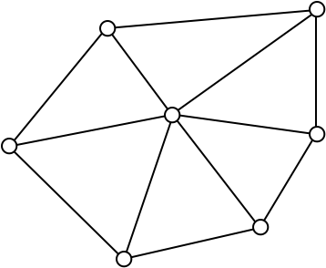
What is a triangle mesh?
- Connectivity / Topology
- Vertices \(\mathcal{V} = \{ v_1, \dots, v_n \}\)
- Edges \(\mathcal{E} = \{ e_1, \dots, e_k \}\), \(e_i \in \mathcal{V} \times \mathcal{V}\)
- Faces \(\mathcal{F} = \{ f_1, \dots, f_m \}\), \(f_i \in \mathcal{V} \times \mathcal{V} \times \mathcal{V}\)
- Geometry
- Vertex positions \(\{ \vec{p}_1, \dots, \vec{p}_n \}\), \(\vec{p}_i \in \R^3\)
Triangle Meshes
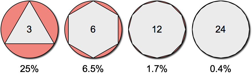
- Triangle meshes can represent arbitrary surfaces

Triangle Meshes
- Triangle meshes can represent arbitrary surfaces
- Piecewise linear approximation → error is \(\mathcal{O}(h^2)\)
Triangle Meshes
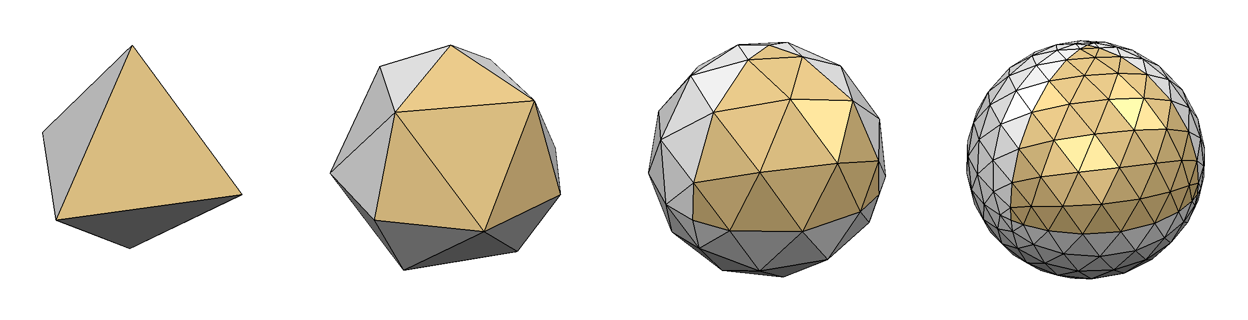
- Triangle meshes can represent arbitrary surfaces
- Piecewise linear approximation → error is \(\mathcal{O}(h^2)\)
- Approximation error inversely proportional to #triangles
Triangle Meshes
- Triangle meshes can represent arbitrary surfaces
- Piecewise linear approximation → error is \(\mathcal{O}(h^2)\)
- Approximation error inversely proportional to #triangles
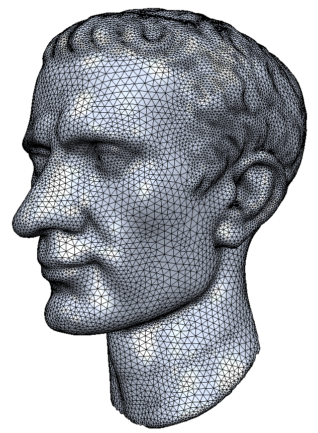
- Adaptive tesselation can adapt to surface curvature
 adaptive meshing
 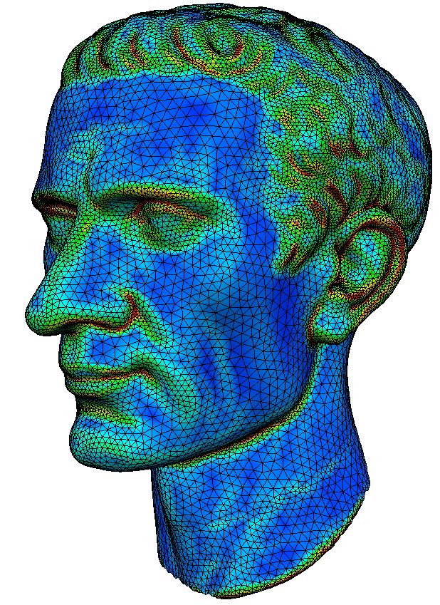 curvature visualization
Triangle Meshes
- Triangle meshes can represent arbitrary surfaces
- Piecewise linear approximation → error is \(\mathcal{O}(h^2)\)
- Approximation error inversely proportional to #triangles
- Adaptive tesselation can adapt to surface curvature
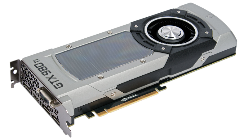
- Simple primitives can be processed efficiently by CPU/GPU

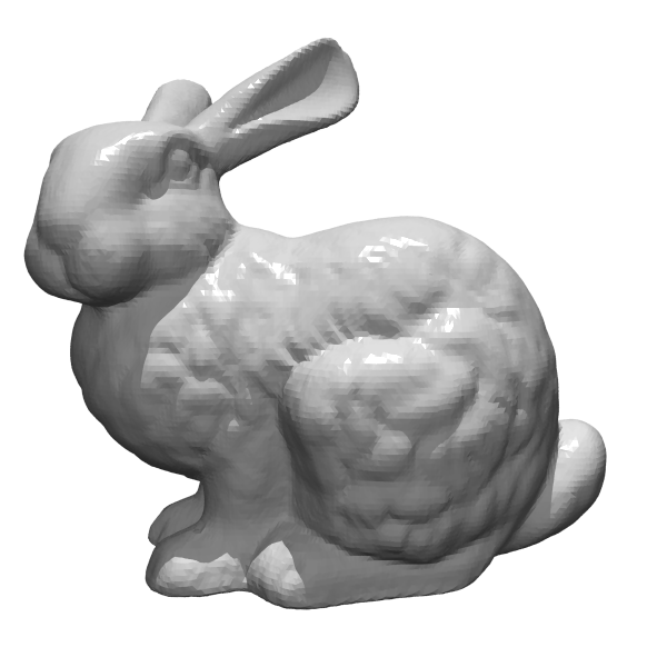
Example: Stanford Bunny
- Observation:
- roughly twice as many faces as vertices
- roughly three times as many edges as vertices
- Coincidence?
- No!
- Euler Formula for meshes of genus 0 \[V - E + F = 2\]
- more on this in the course 3D Geometry Processing (spring)
Face Set
- Face Set is a standard file format for triangle meshes (e.g. STL format)
- Memory consumption
36 B/f = 72 B/v- recall: ~twice as many faces as vertices

Indexed Face Set
- Indexed Face Sets are used for many file formats (e.g. OFF, OBJ, VRML)
- Memory consumption
12 B/v + 12 B/f = 36 B/v

Face-Based Connectivity
- Store connectivity per face
- Memory consumption
16 B/v + 24 B/f = 64 B/v - Non-constant element size for general polygonal meshes
- Edges not represented

Edge-Based Connectivity
- Store connectivity per edge
- Memory consumption
16 B/v + 4 B/f + 32 B/e = 120 B/v - Edges explicitly represented
- Missing edge orientation leads to case distinctions during traversal

Halfedge-Based Connectivity
- Store connectivity per halfedge
- Memory consumption
16 B/v + 4 B/f + 20 B/h = 144 B/v
(can be reduced to 96 B/v) - Edges & halfedges explicitly represented
- No case distinctions during traversal!

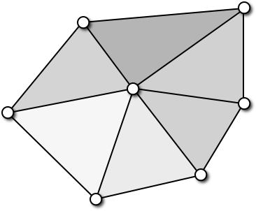
One-Ring Traversal
- Simple one-ring traversal without case distinctions:
- Start at vertex
- Outgoing halfedge
- Opposite halfedge
- Next halfedge
- Opposite halfedge
- Next halfedge
- …

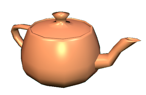
Ray Tracing Meshes
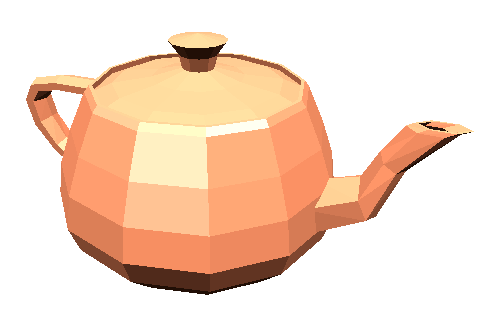
 We want this… …but we get this
Flat Shading vs. Phong Shading
- Flat shading
- Use constant face normal for lighting
- Yields facetted appearence
- Mach band effect emphasizes this even more
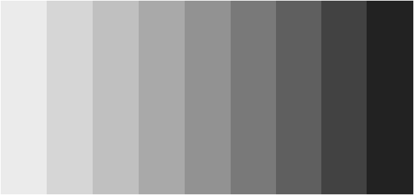 Mach band effect
  source Wikipedia
Flat Shading vs. Phong Shading
- Flat shading
- Use constant face normal for lighting
- Yields facetted appearence
- Mach band effect emphasizes this even more
- Phong shading
- Use smooth normal field for lighting
- Compute normal vectors per vertex
- Barycentric interpolation of normal vectors
Normal Vectors
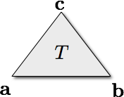
- Triangle normal
\[ \vec{n}(T) = \frac{\left(\vec{b}-\vec{a}\right) \times \left(\vec{c}-\vec{a}\right)} {\norm{\left(\vec{b}-\vec{a}\right) \times \left(\vec{c}-\vec{a}\right)}} \]
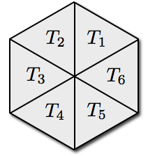
- Vertex normal
- Average of incident triangles’ normals \(\vec{n}(T_i)\)
- Weighted by area or opening angle \(w(T_i)\)
\[ \vec{n}(V) = \frac{ \sum_{T_i \ni V} w(T_i) \, \vec{n}(T_i)} { \norm{ \sum_{T_i \ni V} w(T_i) \, \vec{n}(T_i)} } \]
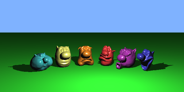
Vertex Normals
 triangulation (flat shading)
  no weighting
 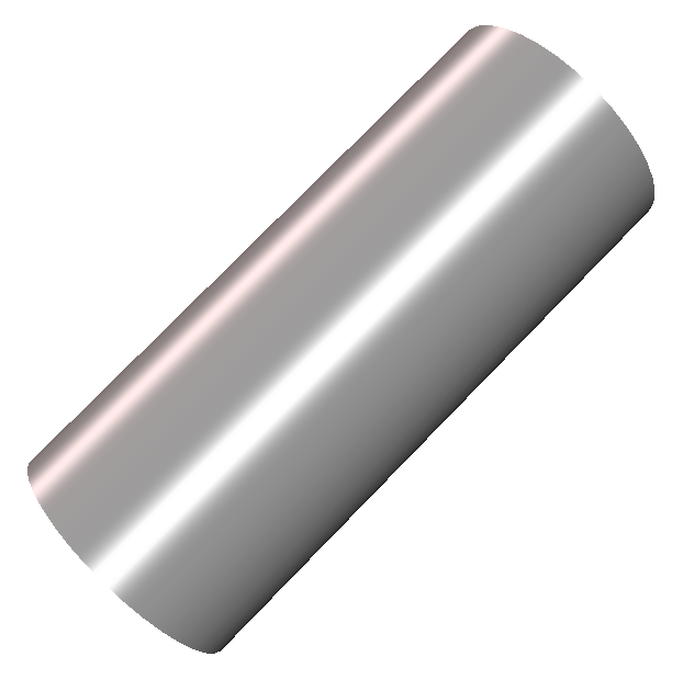 angle-weighted
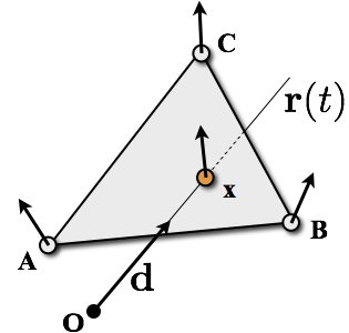
Interpolate Vertex Normals
- Intersection point with barycentric coordinates \[ \vec{x} = \alpha\vec{A} + \beta\vec{B} + \gamma\vec{C}\]
- Linearly interpolate vertex normals \[ \vec{n}\of{\vec{x}} = \alpha\vec{n}\of{\vec{A}} + \beta\vec{n}\of{\vec{B}} + \gamma\vec{n}\of{\vec{C}} \]
- Use \(\vec{n}(\vec{x})\) to light point \(\vec{x}\)
- Normalize for lighting calculations!
Ray Tracing Meshes
Flat Shading Phong Shading
Ray Tracing Meshes
 Flat Shading
 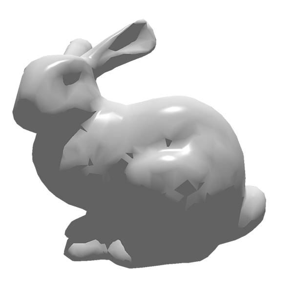 Phong Shading
Ray-Mesh Intersections
- Brute-Force
- Intersect ray with all \(n\) mesh triangles
- Select intersection with smallest positive ray parameter \(t\)
- Computational cost: \(\mathcal{O}(n)\) for single ray
- Many unnecessary ray-triangle intersection tests

KD-Trees
KD-Trees
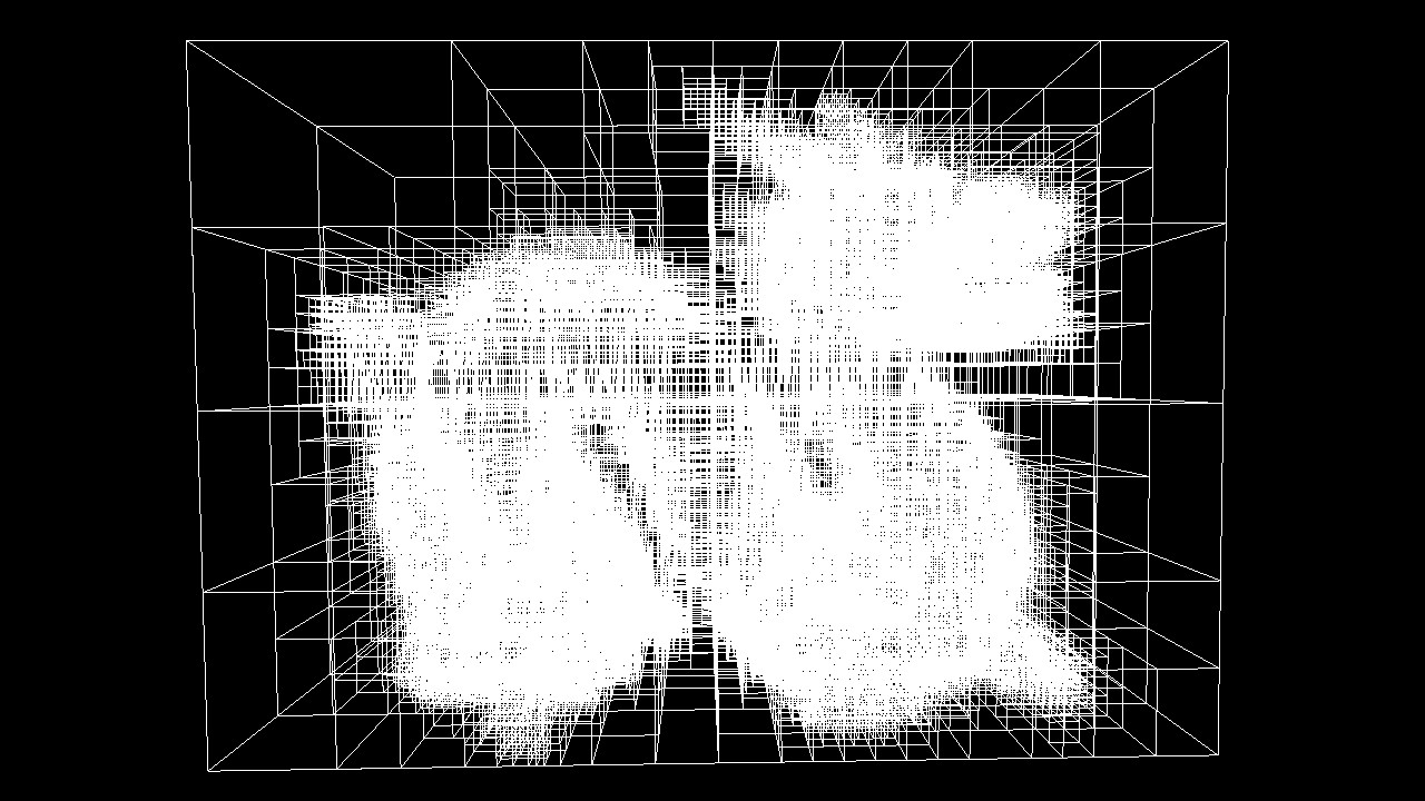
KD-Trees

Axis-Aligned Bounding Boxes
- AABBs are simple to code, but quite effective (see exercises)
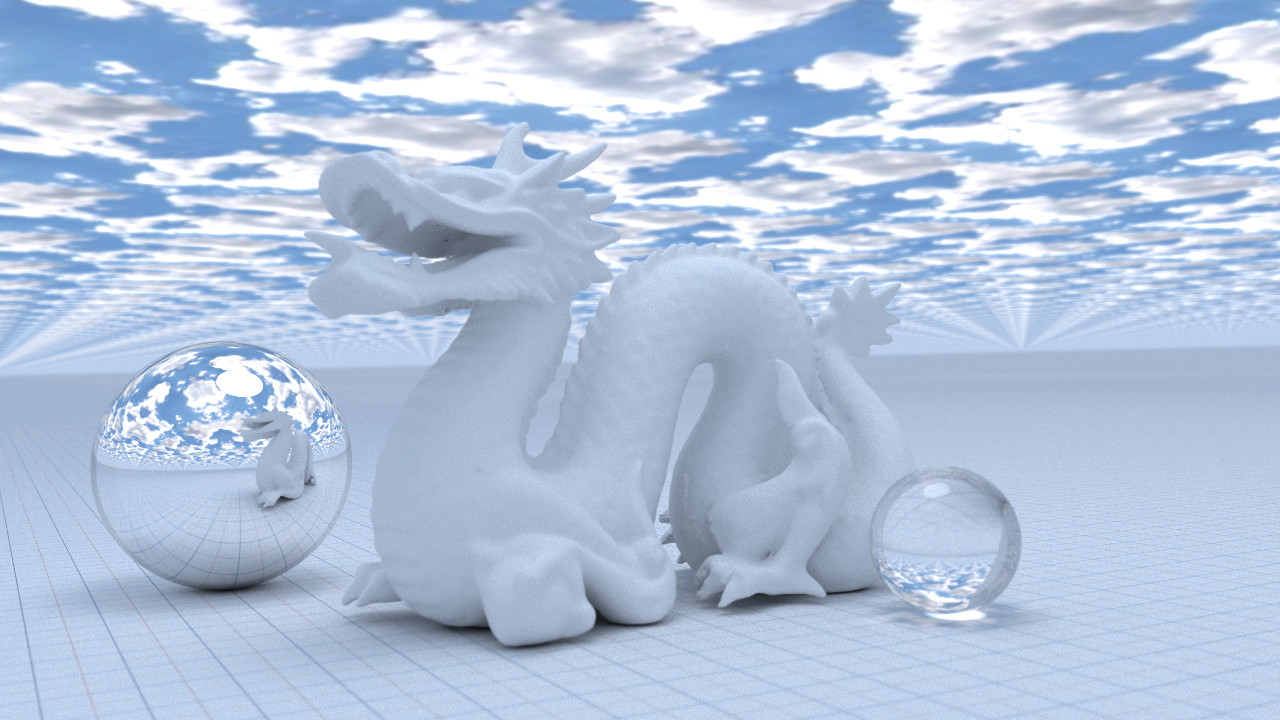
The Quest for Realism
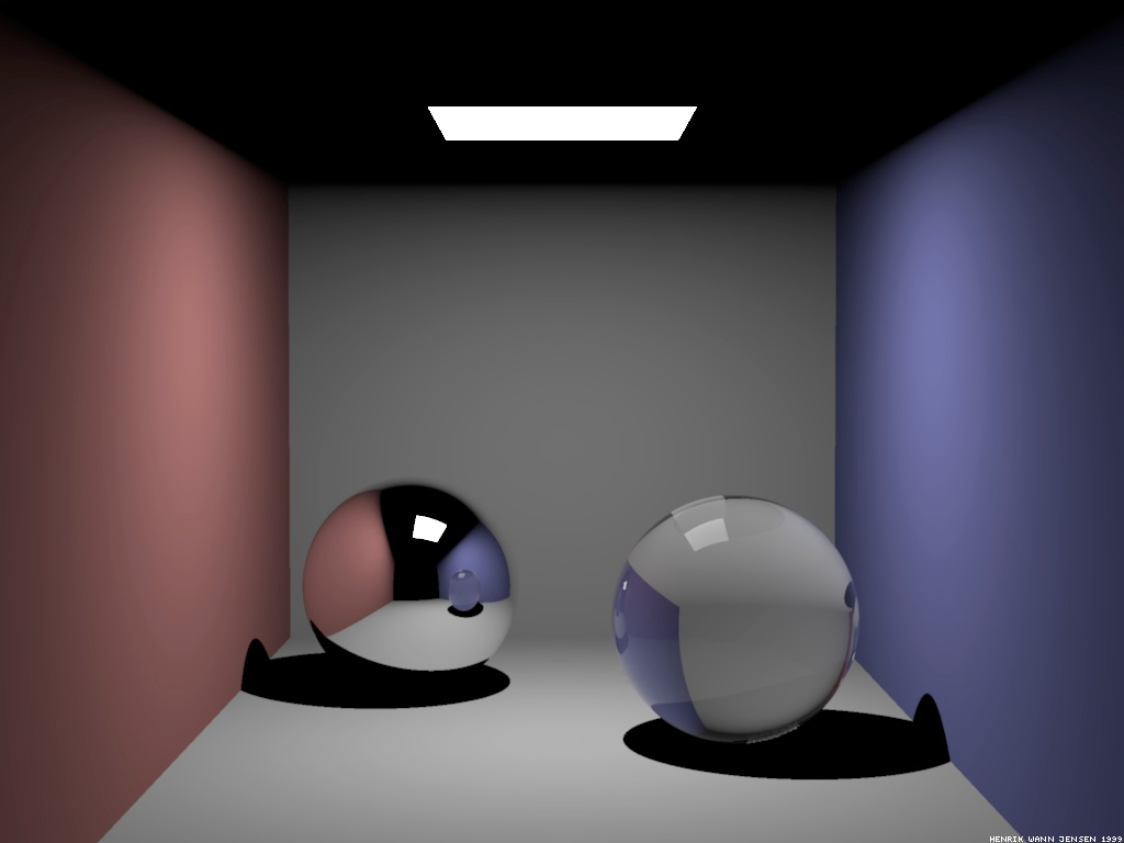 standard ray tracing
 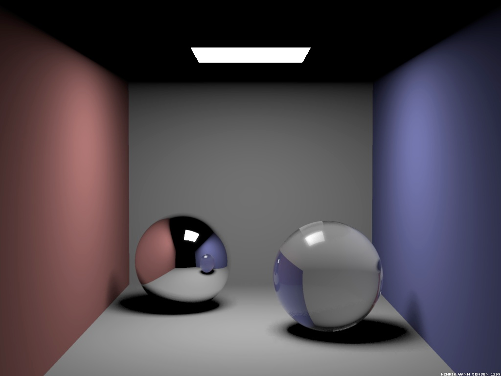 +soft shadows
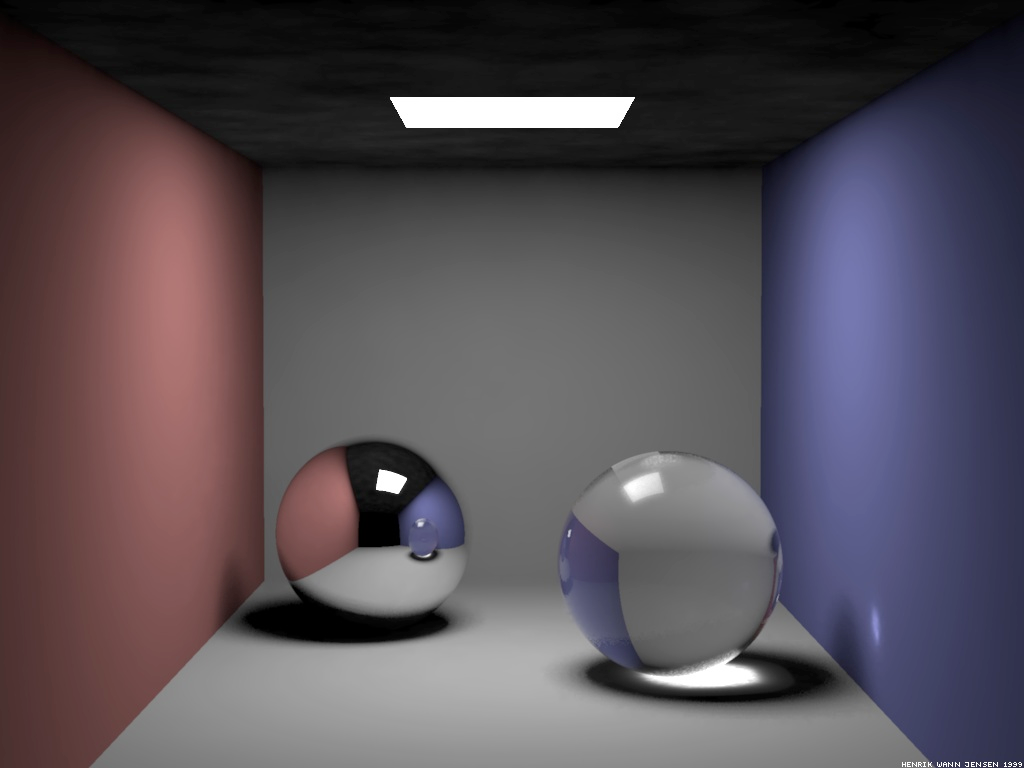 +caustics
 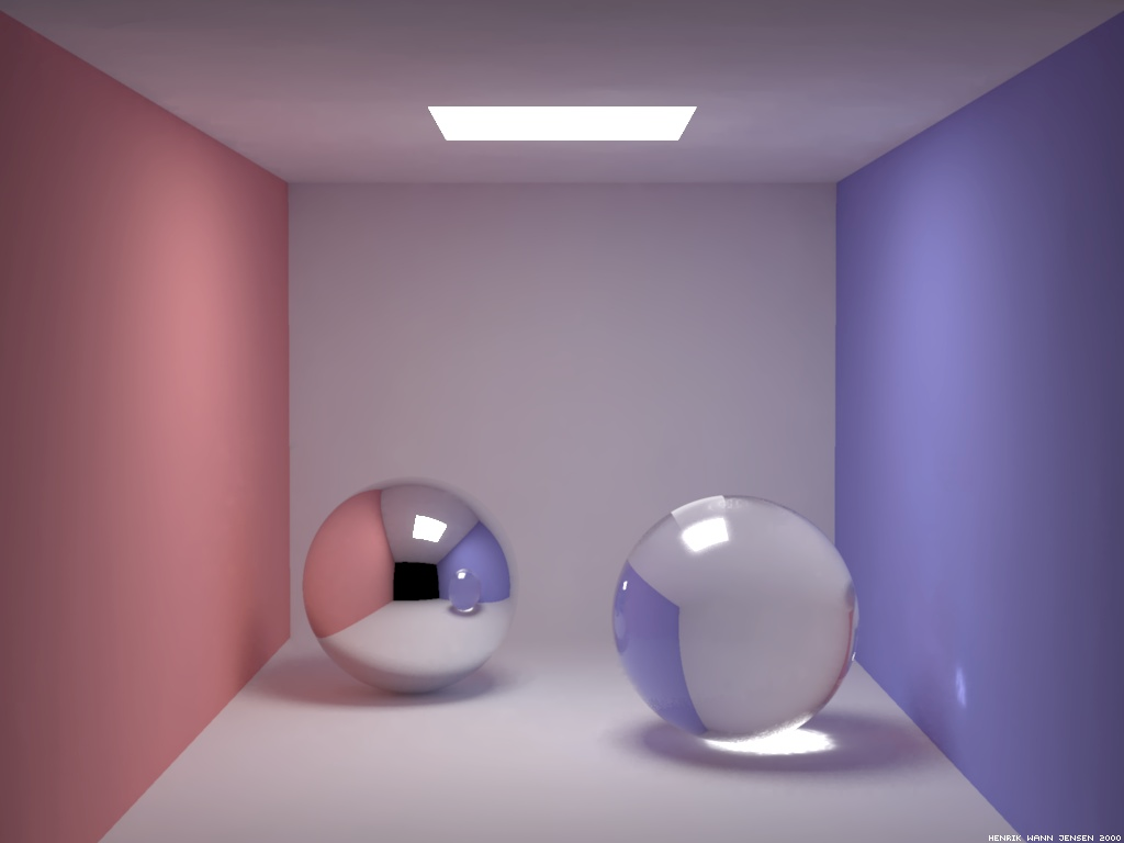 +indirect lighting
Types of Reflections
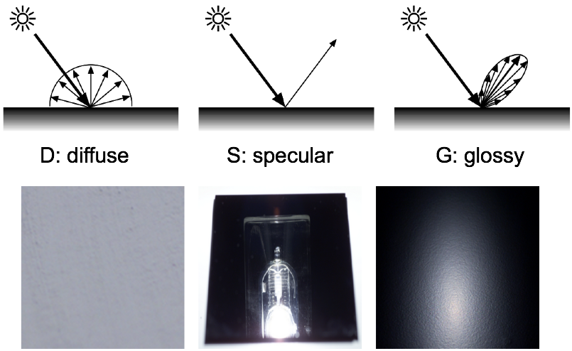
Recursive Ray Tracing
Which light paths can a standard recursive ray-tracer handle?
- Only \(E[S^*](D|G)L\)
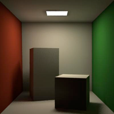
- No multiple diffuse inter-reflections
- E.g. \(EDDL\)
- No caustics
- E.g. \(EDSL\)

Literature
- Botsch, Kobbelt, Pauly, Alliez, Levy: Polygon Mesh Processing, AK Peteres, 2010.
- Chapters 1.3 and 2
- Pharr, Humphreys: Physically Based Rendering, Morgan Kaufmann, 2004.
- Chapter 3
- Hughes et al.: Computer Graphics: Principles and Practice, 3rd Edition, Addison-Wesley, 2014.
- Chapters 25, 37