Computer Graphics
Lighting


Ray Tracing Operators


Ray Tracing Operators

Ray Equation
- Explicit equation for ray \(\vec{r}(t)\), starting at origin \(\vec{o}\)
and going in (normalized) direction \(\vec{d}\):
\[ \vec{r}(t) = \vec{o} + t \, \vec{d} \]

Ray Tracing Operators

Ray-Sphere Intersection
- Implicit representation of a sphere with center \(\vec{c}\) and radius \(r\): \[ \norm{ \vec{x} - \vec{c} } - r = 0 \]

- Insert explicit ray equation into implicit sphere equation: \[ \norm{ \vec{o} + t\vec{d} - \vec{c} } - r = 0 \] and solve for \(t\).
Ray-Plane Equation
- Implicit equation for a plane with normal \(\vec{n}\) and distance \(d\) from origin: \[ \transpose{\vec{n}} \vec{x} - d = 0 \]

- Insert explicit ray equation into implicit plane equation \[ \transpose{\vec{n}} \left(\vec{o} + t\,\vec{d} \right) - d = 0 \] and solve for \(t\).
Ray-Triangle Intersection (explicit)
- Ray and triangle have to coincide \[ \vec{o} + t\,\vec{d} \;=\; \alpha\vec{A} + \beta\vec{B} + \gamma\vec{C}\] Four unknowns, but only three equations!
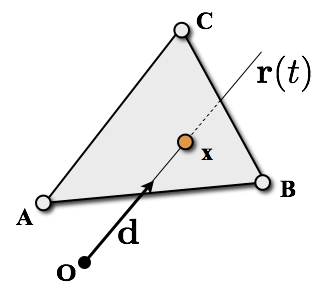
- Exploit condition \(\alpha+\beta+\gamma=1\) to eleminate \(\alpha\) \[ \vec{o} + t\,\vec{d} \;=\; (1-\beta-\gamma)\vec{A} + \beta\vec{B} + \gamma\vec{C}\] Solve \(3 \times 3\) linear system (Cramer’s rule)
- Check inside conditions: \(0 \leq \alpha, \beta, \gamma \leq 1\)
Ray Tracing Operators

Quiz: Barycentric Coordinates
What are the barycentric coordinates \((\alpha, \beta, \gamma)\) of point \(P = \alpha A + \beta B + \gamma C\)?

- (0, 0.5, 0.5)
- (1, 1, 0)
- (0.5, 0.5, 0)
Quiz: Barycentric Coordinates
What are the barycentric coordinates \((\alpha, \beta, \gamma)\) of point \(Q = \alpha A + \beta B + \gamma C\)?

- (-1, 1, 1)
- (-1, 0, 2)
- (0, 1.5, -0.5)
Quiz: Barycentric Coordinates
What are the barycentric coordinates \((\alpha, \beta, \gamma)\) of point \(R = \alpha A + \beta B + \gamma C\)?

- (-0.5, 2, -0.5)
- (1, -1, 1)
- (0, -1, 2)
Ray Tracing Operators
Lighting is important!
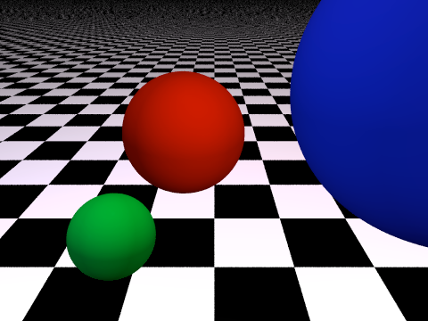
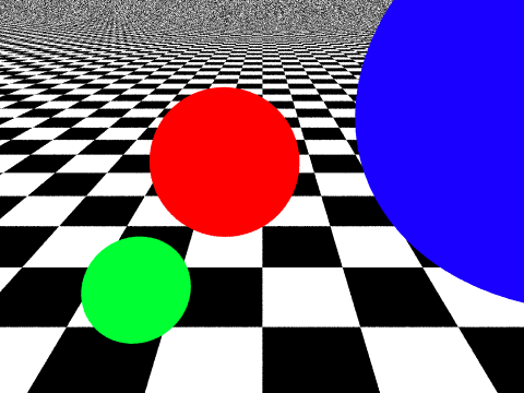 no illumination
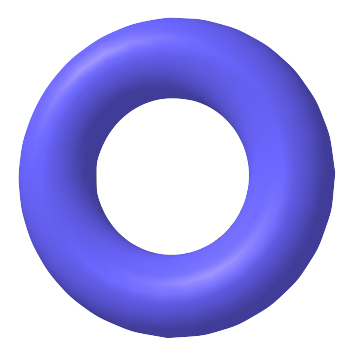
 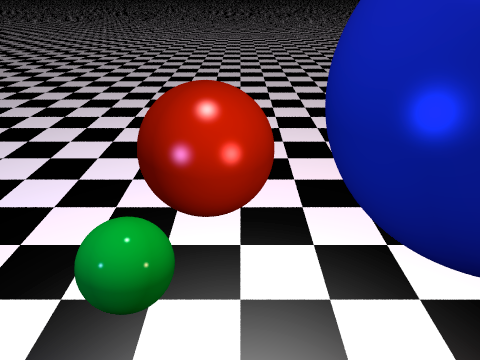 local illumination
 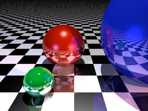 global illumination
Surface Reflectance
- How much light is leaving point \(\vec{x}\) in direction \(\vec{\omega}_{\mathrm{out}}\)?

Surface Reflectance
- How much light is leaving point \(\vec{x}\) in direction \(\vec{\omega}_{\mathrm{out}}\)?

- Collect incoming light \(L_{\mathrm{in}}\) from all directions \(\vec{\omega}_{\mathrm{in}} \in \Omega\) \[ L_{\mathrm{out}}\of{\vec{\omega}_\mathrm{out}} \;=\; \int_{\Omega} \, f(\vec{\omega}_{\mathrm{in}}, \vec{\omega}_{\mathrm{out}}) \, L_{\mathrm{in}}\of{\vec{\omega}_{\mathrm{in}}} \, \cos\of{\theta_{\mathrm{in}}} \, \mathrm{d}\vec{\omega}_{\mathrm{in}} \]
Surface Reflectance
- How much light coming in from direction \(\vec{\omega}_{\mathrm{in}}\) is reflected out in direction \(\vec{\omega}_{\mathrm{out}}\)?

- Determined by the object’s BRDF \(f(\vec{\omega}_{\mathrm{in}}, \vec{\omega}_{\mathrm{out}})\)
- Bidirectional Reflectance Distribution Function
- General description of an object’s material
Phong Lighting Model
- Ambient lighting
- approximate global light transport / exchange
- uniform in, uniform out
- Diffuse lighting
- dull / matt surfaces
- directed in, uniform out
- Specular lighting
- shiny surfaces
- directed in, directed out
Ambient Light

Ambient Light

\[ I \;=\; I_a \, m_a \]
- \(I_a\): ambient light intensity in the scene
- \(m_a\): material’s ambient reflection coefficient
Lighting Computations
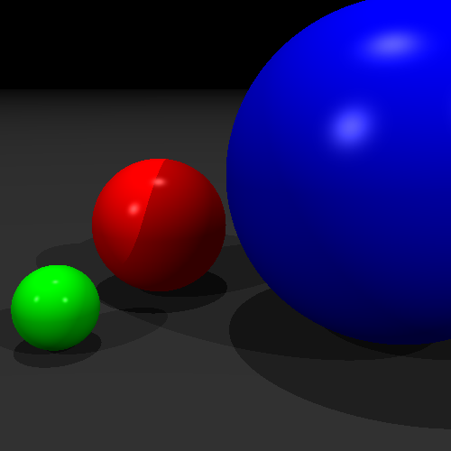
ambient +diffuse +specular 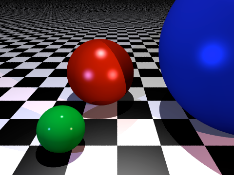 +shadows +reflections
Diffuse Reflection

Diffuse Reflection

Brightness depends on how much light (density) comes in!
Diffuse Reflection


- Intensity inversely proportional to illuminated area
- Illuminated area inversely proportional to \(\cos\of{\theta}\)
- Therefore intensity proportional to \(\cos\of{\theta}\)
- So-called Lambertian reflection
Diffuse Reflection

\[ I \;=\; I_l \, m_d \, \cos\theta \]
- \(I_l\): intensity of light source \(l\)
- \(m_d\): material’s diffuse reflection coefficient
- How can we compute \(\cos\theta\) efficiently?
Diffuse Reflection
\[ I \;=\; I_l \, m_d \, \cos\theta \;=\; I_l \, m_d \, \left( \vec{n} \cdot \vec{l} \right) \]
- \(I_l\): intensity of light source \(l\)
- \(m_d\): material’s diffuse reflection coefficient
- directions \(\vec{n}\) and \(\vec{l}\) assumed to be normalized
- no illumination if \(\vec{n} \cdot \vec{l} < 0\) (why?)
Lighting Computations
ambient +diffuse +specular +shadows +reflections
Specular Reflection

Specular Reflection

Specular Reflection

How to compute reflected ray \(\vec{r}\)?
- \(\vec{r} = \vec{l} + 2 \vec{s}\)
- \(\vec{s} = \vec{n} \left( \vec{n} \cdot \vec{l} \right) - \vec{l}\)
- \(\vec{r} = 2\, \vec{n} \left( \vec{n} \cdot \vec{l} \right) - \vec{l}\)
Specular Reflection
\[ I \;=\; I_l \, m_s \, \cos\of{\alpha} \;=\; I_l \, m_s \, \left( \vec{r} \cdot \vec{v} \right) \]
- \(I_l\): intensity of light source \(l\)
- \(m_s\): material’s specular reflection coefficient
- all directions assumed to be normalized
- no illumination if \(\vec{n} \cdot \vec{l} < 0\) or \(\vec{r} \cdot \vec{v} < 0\)
- How can we control the surface’s shininess?
Specular Reflection
\[ I \;=\; I_l \, m_s \, \cos^s\of{\alpha} \;=\; I_l \, m_s \, \left( \vec{r} \cdot \vec{v} \right)^s \]
- \(I_l\): intensity of light source \(l\)
- \(m_s\): material’s specular reflection coefficient
- all directions assumed to be normalized
- no illumination if \(\vec{n} \cdot \vec{l} < 0\) or \(\vec{r} \cdot \vec{v} < 0\)
- \(s\): cosine exponent controls shininess

Phong Lighting Model
 ambient: \(I_a m_a\)
  diffuse: \(I_l m_d \left( \vec{n} \cdot \vec{l} \right)\)
 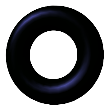 specular: \(I_l m_s \left( \vec{r} \cdot \vec{v} \right)^s\)
\[ I \;=\; I_a m_a + I_l \left( m_d \left( \vec{n} \cdot \vec{l} \right) + m_s \left( \vec{r} \cdot \vec{v} \right)^s \right) \]
Multiple Light Sources
We assumed linear superposition of light contributions and therefore can simply sum over all light sources

\[ I \;=\; I_a m_a + \sum_{l} I_l \left( m_d \left( \vec{n} \cdot \vec{l}_l \right) + m_s \left( \vec{r}_l \cdot \vec{v} \right)^s \right) \]
Lighting Computations
ambient +diffuse +specular +shadows +reflections
Shadows
- Send shadow ray from intersection point to light source.
- Discard diffuse and specular contribution if light source is blocked by another object.


Shadows
- Send shadow ray from intersection point to light source.
- Discard diffuse and specular contribution if light source is blocked by another object.
- Why??
Shadows
- Floating point errors might lead to erroneous self-shadowing (shadow acne).
- Solution 1: Discard secondary intersection points that are too close.
- in our implementation: slightly displace ray origin along new ray direction.
- Solution 2: Offset primary intersection point along surface normal.
- Solution 1: Discard secondary intersection points that are too close.


Lighting Computations
ambient +diffuse +specular +shadows +reflections
Ray Tracing Operators

Recursive Ray Tracing
- At each intersection point, reflect and/or refract incoming viewing ray at surface normal, and trace child rays recursively.
Recursive Ray Tracing
- At each intersection point, reflect and/or refract incoming viewing ray at surface normal, and trace child rays recursively.

\[ \vec{\omega}_{\mathrm{out}} = \left( \mat{I} - 2\vec{n}\transpose{\vec{n}} \right) \vec{\omega}_{\mathrm{in}} \]

\[ n_1 \sin\theta_1 = n_2 \sin\theta_2 \]
Snell’s law with refraction
indices \(n_1\), \(n_2\).
- Remember precision issue: You need to offset ray origin!
Recursive Ray Tracing
At each intersection point, reflect and/or refract incoming viewing ray at surface normal, and trace child rays recursively.
The final color is interpolated between local illumination, reflection, and refraction based on material properties.
Lighting Computations
ambient +diffuse +specular +shadows +reflections
Ray Tracing Pipeline
- Now you know about ray generation, ray intersection, lighting computations, and recursive ray tracing.
- That’s all you need to implement a complete (basic) ray tracer!
- Next week: Raytracing triangle meshes and acceleration data structures
Literature
- Shirley et al.: Fundamentals of Computer Graphics, 3rd Edition, AK Peters, 2009.
- Chapter 10, 20
- Hughes et al.: Computer Graphics: Principles and Practice, 3rd Edition, Addison-Wesley, 2014.
- Chapter 27.5
- Akenine-Möller, Haines, Hoffman: Real-Time Rendering, Taylor & Francis, 2008.
- Chapters 5 and 7