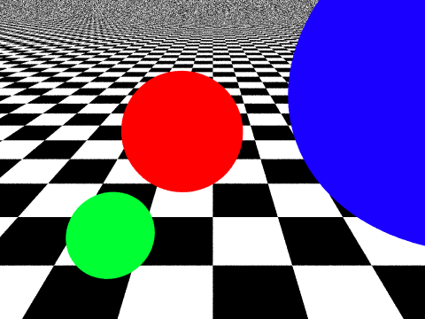
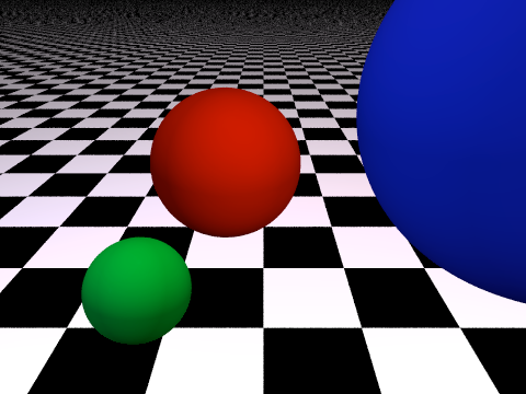
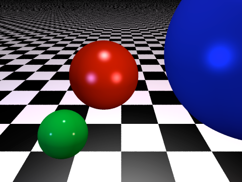
Computer Graphics

Raytracing - Intersections

Prof. Dr. David Bommes

Computer Graphics Group

Part I: Raytracing

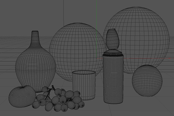
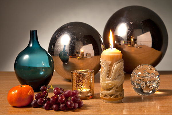
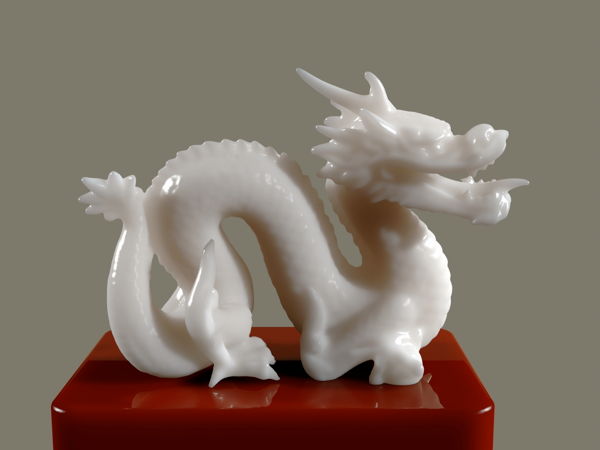
Goal: How to generate realistic digital images of synthetic 3D scenes?

images/wireframe.jpg images/photoreal.jpg

Image Source

Part I: Raytracing

Goal: How to generate realistic digital images of synthetic 3D scenes?
Several questions arise:
- What is light?
- How is light propagated?
- How does light interact with objects?
- How does a camera work?

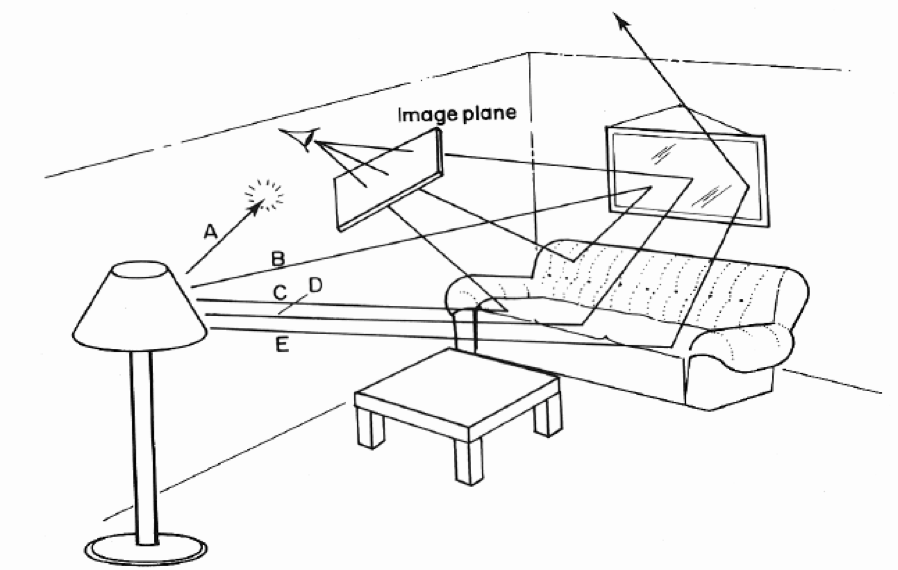
Light Transport

Light Transport Assumptions

Geometric optics
Light propagates along rays, not waves
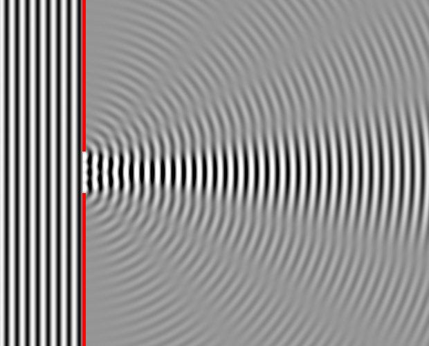
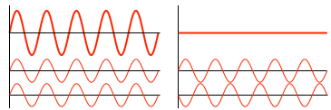
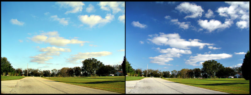
$\Rightarrow$ no diffraction, no interference, no polarization

$images/diffraction.png$ diffraction images/interference.png interference images/polarization.png polarization Images from Wikipedia

Light Transport Assumptions

Geometric optics
Light propagates along rays, not waves
$\Rightarrow$ no diffraction, no interference, no polarization
RGB approximation
Approximate light spectrum by discrete RGB wavelengths
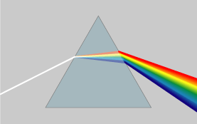
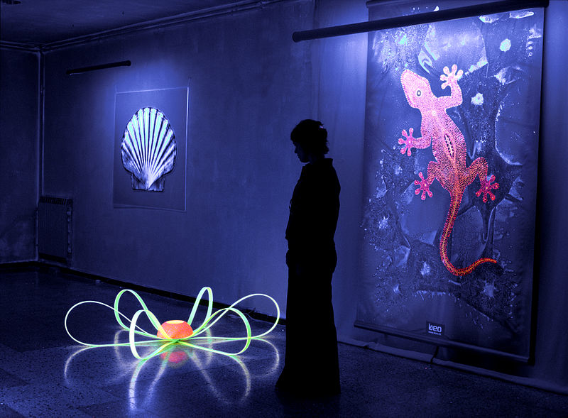
$\Rightarrow$ no dispersion, no fluorescence

images/dispersion.png dispersion images/fluorescence.png fluorescence Images from Wikipedia

Light Transport Assumptions

Geometric optics
Light propagates along rays, not waves
$\Rightarrow$ no diffraction, no interference, no polarization
RGB approximation
Approximate light spectrum by discrete RGB wavelengths
$\Rightarrow$ no dispersion, no fluorescence
No participating media
Light travels along straight rays through vacuum
$\Rightarrow$ no atmospheric scattering, no gravity effects
Superposition
Simply add multiple light contributions
$\Rightarrow$ No nonlinearly reflecting materials

Rendering or Photograph?

images/rendering_vs_photo_quiz/pancakes_cg.jpg cgtrader.com

Rendering
Photo

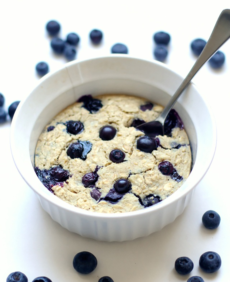
Rendering or Photograph?

images/rendering_vs_photo_quiz/blueberry_muffin_real.jpg cgtrader.com

Rendering
Photo

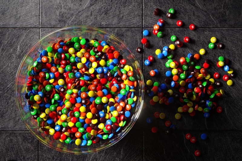
Rendering or Photograph?

images/rendering_vs_photo_quiz/mms_cg.jpg cgtrader.com

Rendering
Photo

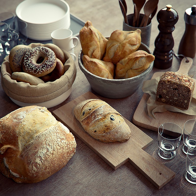
Rendering or Photograph?

images/rendering_vs_photo_quiz/bread_cg.jpg cgtrader.com

Rendering
Photo

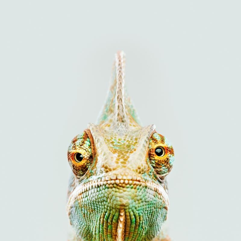
Rendering or Photograph?

images/rendering_vs_photo_quiz/lizard_real.jpg Autodesk

Rendering
Photo

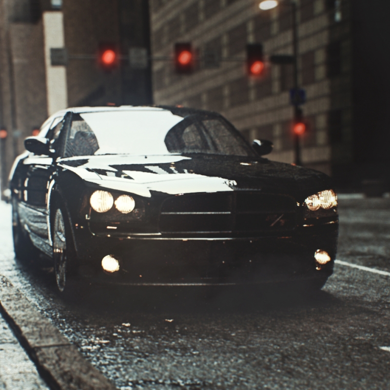
Rendering or Photograph?

images/rendering_vs_photo_quiz/car_cg.jpg Autodesk

Rendering
Photo

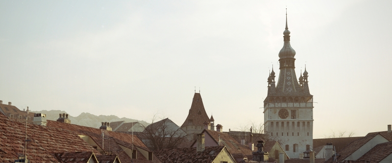
Rendering or Photograph?

images/rendering_vs_photo_quiz/buildings_cg.jpg Autodesk

Rendering
Photo

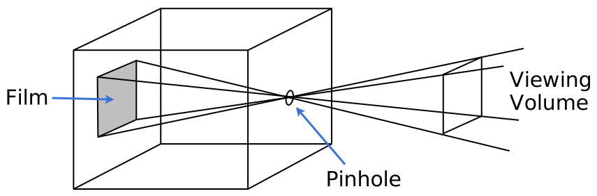
Pinhole Camera

We assume a classical pinhole camera

Pinhole Camera

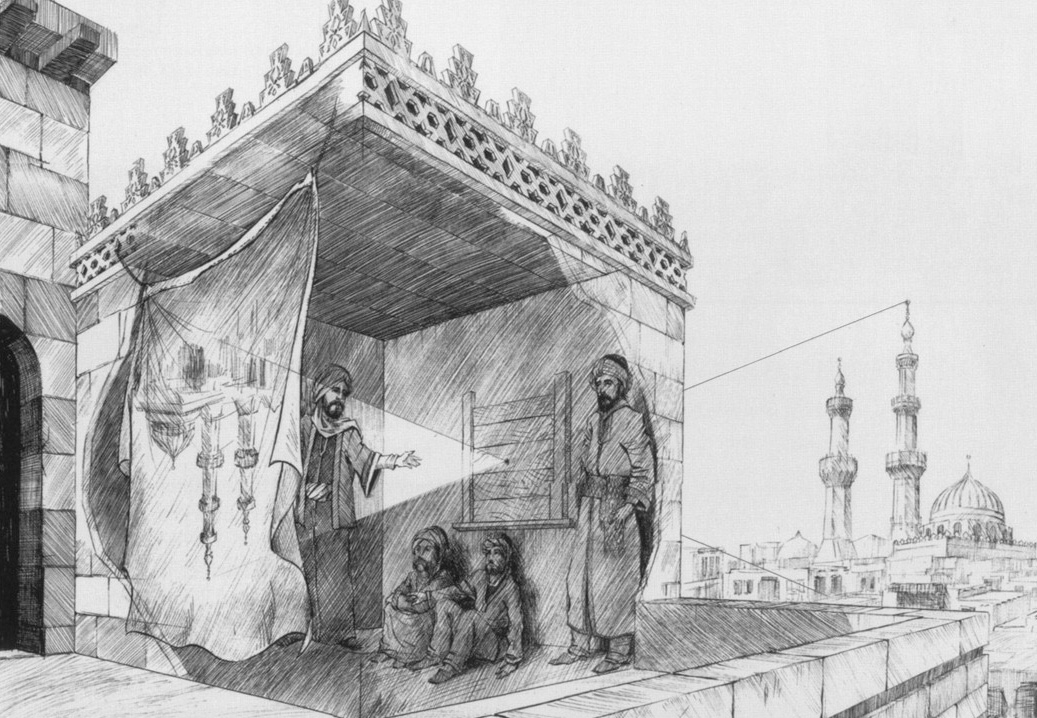
Studied extensively throughout history
Application: Camera Obscura

Mo Tzu (c. 470–c. 390 BC)
Aristotle (384–322 BC)
Ibn al-Haytham (965–1040)
Shen Kuo (1031–1095)
Roger Bacon (c. 1214–1294)
Johannes Kepler (1571–1630)

Source: A. H. Zewail,Phil. Trans. R. Soc. A 2010;368:1191-1204

Pinhole Camera

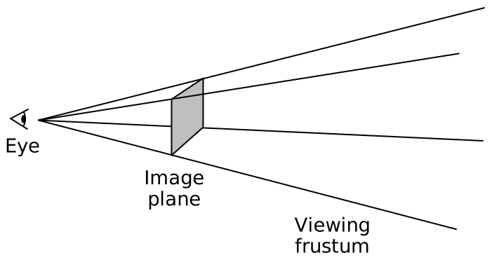
We represent the camera using eye point (pinhole) and image plane (mirrored film)

Forward Ray Tracing

What’s the problem with this approach?

Backward Ray Tracing

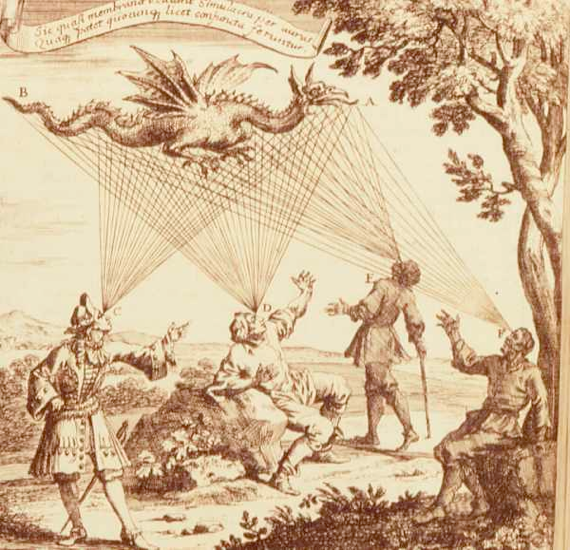
Ancient Greeks - Emission Theory

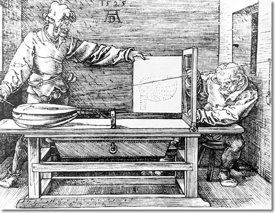
Albrecht Dürer (1525)

images/duerer-1.png — Raycasting Machine

Images from Wikipedia

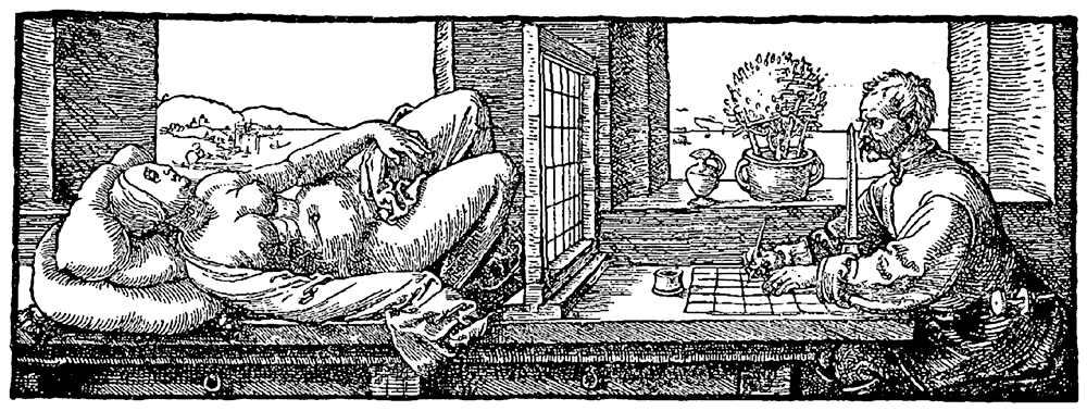
Albrecht Dürer (1525)

Images from Wikipedia

Turner Whitted (1979)

ACM SIGGRAPH 1979 - An improved illumination model for shaded display

Examples from PBRT

images/pbrt-1.png images/pbrt-2.png
images/pbrt-3.png images/pbrt-4.png

http://www.pbrt.org/gallery.html

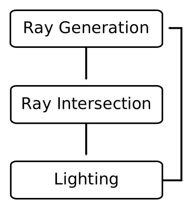
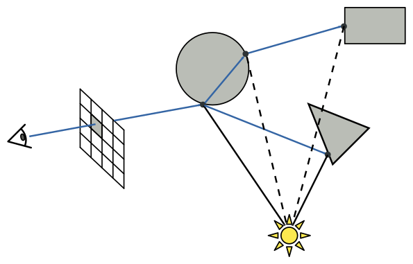
Basic Ray Tracing Pipeline

Implementing a ray tracer basically comes down to
three operators that we have to understand and implement.

images/ray-tracing-pipeline.svg images/ray-tracing.svg

Ray Tracing Pseudo Code

void raytrace()
{
    for (int x=0; x<width; ++x)
    {
        for (int y=0; y<height; ++y)
        {
            // generate primary ray through pixel (x,y)
            ray = primary_ray(x,y);

            // determine color through (recursive!) trace function
            color[x,y] = trace(ray);
        }
    }
}

Ray Generation

Ray Equation

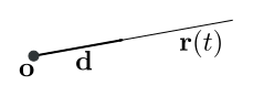
Explicit equation for ray $\vec{r}(t)$, starting at origin $\vec{o}$
and going in (normalized) direction $\vec{d}$:

\[ \vec{r}(t) = \vec{o} + t \, \vec{d} \]

Vector Space $\R^n$

Scalars $\alpha, \beta, \gamma \in \R$ are written in italic (mostly Greek) font.
Vectors $\vec{x}, \vec{y} \in \R^n$ are written in bold font, their components are denoted as $\vec{x}=\transpose{(x_1, \dots, x_n)}$.
Linear combinations $\alpha\,\vec{x} + \beta\,\vec{y}$ stay in vector space and are performed component-wise.

Euclidean Vector Space $\R^n$

Inner product (or scalar product, or dot product) \[ \iprod{ \vec{x} , \vec{y} } = \transpose{\vec{x}}\vec{y} = \vec{x} \cdot \vec{y} = \sum_{i=1}^{n} x_i y_i \] is symmetric and linear in both arguments
The induced metric measures geometric length \[ \norm{\vec{x}} = \sqrt{ \transpose{\vec{x}}\vec{x}} = \left( \sum_{i=1}^n x_i^2 \right)^{\frac{1}{2}}\]
Scalar product can measure angle $\theta$ between two vectors \[ \transpose{\vec{x}} \vec{y} = \cos\theta \, \norm{\vec{x}} \, \norm{\vec{y}} \Rightarrow \theta = \mathrm{acos}\!\left( \frac{\transpose{\vec{x}} \vec{y}}{\norm{\vec{x}} \norm{\vec{y}}}\right)\]

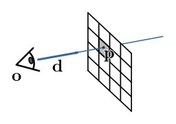
Primary Rays

Shoot a primary ray through each pixel $(x,y)$ of the image plane:

use eye point as origin $\vec{o}$
compute 3D position $\vec{p}$ of pixel $(x,y)$
compute direction $\vec{d} = \frac{\vec{p}-\vec{o}}{\norm{\vec{p}-\vec{o}}}$

Ray Intersection

Ray-Object Intersections

Which surface types or surface primitives do we want to support?
Which properties should surface primitives have?
Spheres, cylinders, planes, boxes, triangles…

Ray-Sphere Intersection

How to represent a sphere?
How to intersect a ray and a sphere?

Unit Sphere

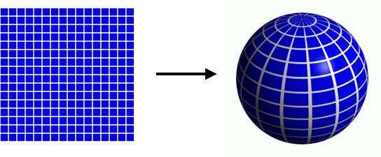
Unit sphere parameterized by spherical coordinates:

\[ \vector{ \phi \\ \theta } \mapsto \vector{ \cos\phi \, \cos\theta \\ \sin\phi \, \cos\theta \\ \sin\theta } \]

Arbitrary Sphere

Sphere with center $\vec{c}$ and radius $r$:

\[ \vector{ \phi \\ \theta } \mapsto \vec{c} + r \, \vector{ \cos\phi \, \cos\theta \\ \sin\phi \, \cos\theta \\ \sin\theta } \]

Ray-Sphere Intersection

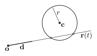
Ray and sphere have to coincide, leading to this equation \[ \vec{o} + t\,\vec{d} = \vec{c} + r \, \vector{ \cos\phi \, \cos\theta \\ \sin\phi \, \cos\theta \\ \sin\theta } \]
which we have to solve for $t$, $\phi$, and $\theta$.

Trigonometric functions make this
equation nonlinear and complicated!

Ray-Sphere Intersection, 2nd try

Let us use the implicit representation of a sphere with center $\vec{c}$ and radius $r$: \[ \norm{ \vec{x} - \vec{c} } - r = 0 \]
This equation is satisfied by all points $\vec{x} \in \R^3$ that lie on the sphere.

Insert explicit ray equation into implicit sphere equation: \[ \norm{ \vec{o} + t\vec{d} - \vec{c} } - r = 0 \]
and solve for $t$. Much easier and more efficient!

Ray-Plane Intersection

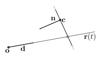
Implicit equation for a plane with normal $\vec{n}$ centered at point $\vec{c}$ (or with distance $d$ from origin): \[ \begin{eqnarray*} \transpose{\vec{n}} \left( \vec{x} - \vec{c} \right) &=& 0 \\ \transpose{\vec{n}} \vec{x} - d &=& 0 \end{eqnarray*} \]

Insert explicit ray equation into implicit plane equation \[ \transpose{\vec{n}} \left(\vec{o} + t\,\vec{d} \right) - d = 0 \]
and solve for $t$.

Ray-Triangle Intersection

How can we represent a triangle?
Should we rather use an implicit or explicit formulation?
Which one can be intersected with a ray more efficiently?

Ray-Triangle Intersection (implicit version)

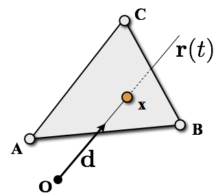
Construct triangle’s supporting plane

3D Cross Product

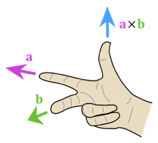
Given two 3D vectors $\vec{a}$ and $\vec{b}$, finds a vector $\vec{c}$ that is orthogonal to them \[ \vec{c} \;=\; \vec{a} \times \vec{b} \;=\; {\tiny \matrix{ a_2 b_3 - a_3 b_2 \\ a_3 b_1 - a_1 b_3 \\ a_1 b_2 - a_2 b_1 }} \]

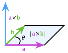
Measures the area of parallelogram spanned by vectors $\vec{a}$ and $\vec{b}$ \[ \norm{\vec{a} \times \vec{b}} = \norm{\vec{a}} \cdot \norm{\vec{b}} \cdot \sin\theta \]

Measures volume spanned by vectors $\vec{a}$, $\vec{b}$, $\vec{c}$ \[ \mathrm{vol}\of{\vec{a}, \vec{b}, \vec{c}} \;=\; \abs{ \vec{a} \, \vec{b} \, \vec{c} } \;=\; \transpose{\left( \vec{a} \times \vec{b} \right)} \vec{c} \]

Images from Wikipedia

Ray-Triangle Intersection (implicit version)

Construct triangle’s supporting plane
- Normal $\vec{n} = \frac{(\vec{B}-\vec{A}) \times (\vec{C}-\vec{A})} {\norm{(\vec{B}-\vec{A}) \times (\vec{C}-\vec{A})}}$
- Distance from origin $d = \transpose{\vec{n}}\vec{A} = \transpose{\vec{n}}\vec{B} = \transpose{\vec{n}}\vec{C}$
Intersect ray with triangle’s plane
- Solve $\transpose{(\vec{o} + t\vec{d})}\vec{n} - d = 0$
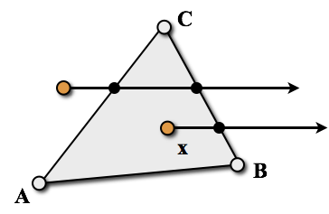
Is intersection point inside/outside of triangle?
- Project to 2D coordinates
- Point-in-polygon test

images/ray-triangle-intersection.png

Barycentric Coordinates

Explicit triangle parameterization (first guess)
- Origin $\vec{A}$, edges $\vec{U} = \vec{B}-\vec{A}$ and $\vec{V} = \vec{C}-\vec{A}$
- Triangle points $\vec{x} = \vec{A} + u\,\vec{U} + v\,\vec{V}$
  with $u,v \geq 0$ and $u+v\leq 1$

Barycentric coordinates (more useful later)
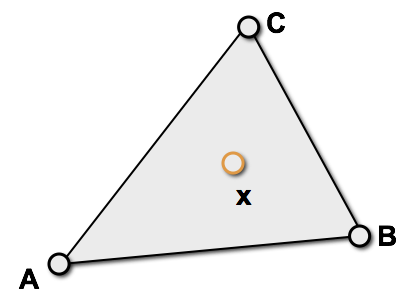
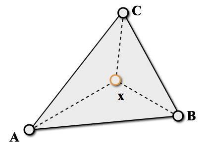
- $\vec{x} = \alpha\vec{A} + \beta\vec{B} + \gamma\vec{C}$
  with $\alpha + \beta + \gamma = 1$ and $\alpha,\beta,\gamma \geq 0$.
- Equivalent to above (why?)

Barycentric Coordinates

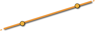
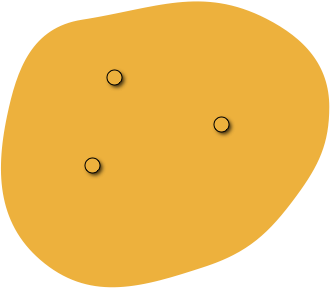
Affine combination of two points \[\vec{x} = \alpha\vec{A} + \beta\vec{B}\]
with $\alpha + \beta = 1$.

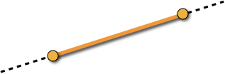
Convex combination of two points \[\vec{x} = \alpha\vec{A} + \beta\vec{B}\]
with $\alpha + \beta = 1$ and $\alpha,\beta \geq 0$.

Barycentric Coordinates

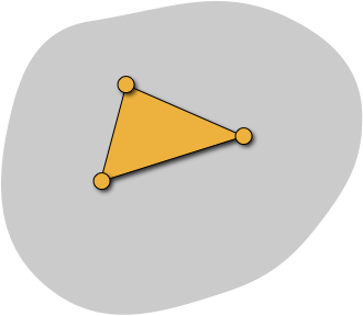
Affine combination of three points \[\vec{x} = \alpha\vec{A} + \beta\vec{B} + \gamma\vec{C}\]
with $\alpha + \beta + \gamma = 1$.

Convex combination of three points \[\vec{x} = \alpha\vec{A} + \beta\vec{B} + \gamma\vec{C}\]
with $\alpha + \beta + \gamma = 1$ and $\alpha,\beta,\gamma \geq 0$.

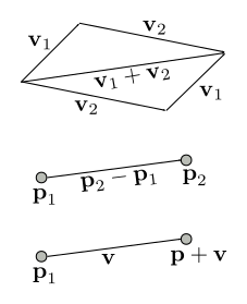
Points vs. Vectors

Subtle distinction
- Points denote positions in $\R^3$
- Vectors denote differences of points

Meaningful operations
- vector + vector = vector
- point - point = vector
- point + vector = point
- point + point = ???

Barycentric Coordinates

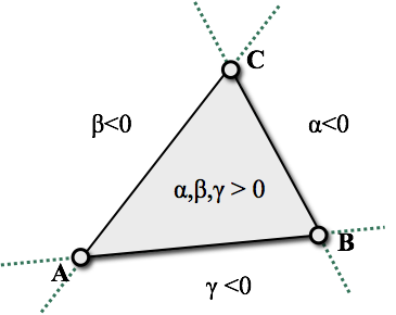
Ratio of (signed!) areas (volumes in 3D) \[ \begin{eqnarray*} \alpha\of{\vec{x}} &=& \mathrm{area}\of{\vec{x}, \vec{B}, \vec{C}} /\, \mathrm{area}\of{\vec{A}, \vec{B}, \vec{C}} \\ \beta\of{\vec{x}} &=& \mathrm{area}\of{\vec{A}, \vec{x}, \vec{C}} /\, \mathrm{area}\of{\vec{A}, \vec{B}, \vec{C}} \\ \gamma\of{\vec{x}} &=& \mathrm{area}\of{\vec{A}, \vec{B}, \vec{x}} /\, \mathrm{area}\of{\vec{A}, \vec{B}, \vec{C}} \end{eqnarray*} \]

Gives the required inside/outside information!

Ray-Triangle Intersection (explicit)

Ray and triangle have to coincide \[ \vec{o} + t\,\vec{d} \;=\; \alpha\vec{A} + \beta\vec{B} + \gamma\vec{C}\]
Four unknowns, but only three equations!

Exploit condition $\alpha+\beta+\gamma=1$ to eleminate $\alpha$ \[ \vec{o} + t\,\vec{d} \;=\; (1-\beta-\gamma)\vec{A} + \beta\vec{B} + \gamma\vec{C}\]
Solve $3 \times 3$ linear system (Cramer’s rule)

Check inside conditions: $0 \leq \alpha, \beta, \gamma \leq 1$

Other Primitives

Cylinder (exercise)
Cone, paraboloid, hyperboloid
Meshes (in two weeks)
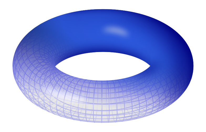
Torus

\[(R-\sqrt{\vec{x}^2 + \vec{y}^2})^2 + \vec{z}^2 = r^2\]

Wikipedia

Ray Tracing Pipeline

We understood ray generation and ray intersections.
Next week we’ll talk about lighting.

images/ray-tracing-pipeline.svg images/ray-tracing.svg

Ray Tracing Pipeline

We understood ray generation and ray intersections.
Next week we’ll talk about lighting.

images/spheres-0.png color only images/spheres-1.png +diffuse images/spheres-2.png +specular

Is it difficult to code?

Paul Heckbert’s Minimal Ray Tracer
(was printed on the back of his business card)

typedef struct{double x,y,z}vec;vec U,black,amb={.02,.02,.02};struct sphere{
vec cen,color;double rad,kd,ks,kt,kl,ir}*s,*best,sph[]={0.,6.,.5,1.,1.,1.,.9,
.05,.2,.85,0.,1.7,-1.,8.,-.5,1.,.5,.2,1.,.7,.3,0.,.05,1.2,1.,8.,-.5,.1,.8,.8,
1.,.3,.7,0.,0.,1.2,3.,-6.,15.,1.,.8,1.,7.,0.,0.,0.,.6,1.5,-3.,-3.,12.,.8,1.,
1.,5.,0.,0.,0.,.5,1.5,};yx;double u,b,tmin,sqrt(),tan();double vdot(A,B)vec A
,B;{return A.x*B.x+A.y*B.y+A.z*B.z;}vec vcomb(a,A,B)double a;vec A,B;{B.x+=a*
A.x;B.y+=a*A.y;B.z+=a*A.z;return B;}vec vunit(A)vec A;{return vcomb(1./sqrt(
vdot(A,A)),A,black);}struct sphere*intersect(P,D)vec P,D;{best=0;tmin=1e30;s=
sph+5;while(s-->sph)b=vdot(D,U=vcomb(-1.,P,s->cen)),u=b*b-vdot(U,U)+s->rad*s
->rad,u=u>0?sqrt(u):1e31,u=b-u>1e-7?b-u:b+u,tmin=u>=1e-7&&u<tmin?best=s,u:
tmin;return best;}vec trace(level,P,D)vec P,D;{double d,eta,e;vec N,color;
struct sphere*s,*l;if(!level--)return black;if(s=intersect(P,D));else return
amb;color=amb;eta=s->ir;d= -vdot(D,N=vunit(vcomb(-1.,P=vcomb(tmin,D,P),s->cen
)));if(d<0)N=vcomb(-1.,N,black),eta=1/eta,d= -d;l=sph+5;while(l-->sph)if((e=l
->kl*vdot(N,U=vunit(vcomb(-1.,P,l->cen))))>0&&intersect(P,U)==l)color=vcomb(e
,l->color,color);U=s->color;color.x*=U.x;color.y*=U.y;color.z*=U.z;e=1-eta*
eta*(1-d*d);return vcomb(s->kt,e>0?trace(level,P,vcomb(eta,D,vcomb(eta*d-sqrt
(e),N,black))):black,vcomb(s->ks,trace(level,P,vcomb(2*d,N,D)),vcomb(s->kd,
color,vcomb(s->kl,U,black))));}main(){printf("%d %d\n",32,32);while(yx<32*32)
U.x=yx%32-32/2,U.z=32/2-yx++/32,U.y=32/2/tan(25/114.5915590261),U=vcomb(255.,
trace(3,black,vunit(U)),black),printf("%.0f %.0f %.0f\n",U);}/*minray!*/

Literature

Shirley et al.: Fundamentals of Computer Graphics, 3rd Edition, AK Peters, 2009.
- Chapter 4

Glassner: An Introduction to Ray Tracing, Academic Press, 1989.
- Chapters 2 & 4

Pharr, Humphreys: Physically Based Rendering, Morgan Kaufmann, 2004.
- Chapters 1-3

Computer Graphics

Raytracing - Intersections

Part I: Raytracing

Part I: Raytracing

Light Transport

Light Transport Assumptions

Light Transport Assumptions

Light Transport Assumptions

Rendering or Photograph?

Rendering or Photograph?

Rendering or Photograph?

Rendering or Photograph?

Rendering or Photograph?

Rendering or Photograph?

Rendering or Photograph?

Pinhole Camera

Pinhole Camera

Pinhole Camera

Forward Ray Tracing

Backward Ray Tracing

Ancient Greeks - Emission Theory

Albrecht Dürer (1525)

Albrecht Dürer (1525)

Turner Whitted (1979)

Examples from PBRT

Basic Ray Tracing Pipeline

Ray Tracing Pseudo Code

Ray Generation

Ray Equation

Vector Space \(\R^n\)

Euclidean Vector Space \(\R^n\)

Primary Rays

Ray Intersection

Ray-Object Intersections

Ray-Sphere Intersection

Unit Sphere

Arbitrary Sphere

Ray-Sphere Intersection

Ray-Sphere Intersection, 2nd try

Ray-Plane Intersection

Ray-Triangle Intersection

Ray-Triangle Intersection (implicit version)

3D Cross Product

Ray-Triangle Intersection (implicit version)

Barycentric Coordinates

Barycentric Coordinates

Barycentric Coordinates

Points vs. Vectors

Barycentric Coordinates

Ray-Triangle Intersection (explicit)

Other Primitives

Ray Tracing Pipeline

Ray Tracing Pipeline

Is it difficult to code?

Literature